3597
Calgary-Campinas raw k-space dataset: a benchmark for brain magnetic resonance image reconstruction1University of Calgary, Calgary, AB, Canada, 2University of Campinas, Campinas, Brazil
Synopsis
Machine learning is a new frontier for magnetic resonance (MR) image reconstruction, but progress is hampered by a lack of benchmark datasets. Our datasets provides ~200 GB of brain MR data (both raw and reconstructed data) acquired with different acquisition parameters on different scanners from different vendors and different magnetic field intensities. The fastMRI initiative (https://fastmri.org/), also provides raw data but otherwise is complementary. For instance, fastMRI provides raw k-space data corresponding to 2D acquisitions, while our dataset is composed of 3D acquisitions (i.e., with our data, you can under-sample in two directions).
Introduction
Machine learning, especially deep learning, applied to magnetic resonance (MR) image reconstruction is a very active research area.1-15 Advancements in the field however suffer from the lack of benchmark datasets. Thus, most publications use private datasets to assess their results making it difficult to determine the state-of-the-art approach. The fastMRI16 (https://fastmri.org/) initiative helps to reduce this problem. The existing Calgary-Campinas (CC) brain MR dataset17 now complements this initiative. We started in 2016 with the goal of providing a large and heterogenous datasets of T1-weighted volumetric imaging in order to advance methods that analyze brain MR images. Here, we report on an expansion of the CC dataset to include raw k-space data.Materials and Methods
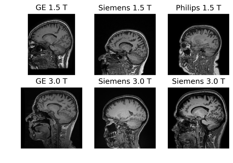
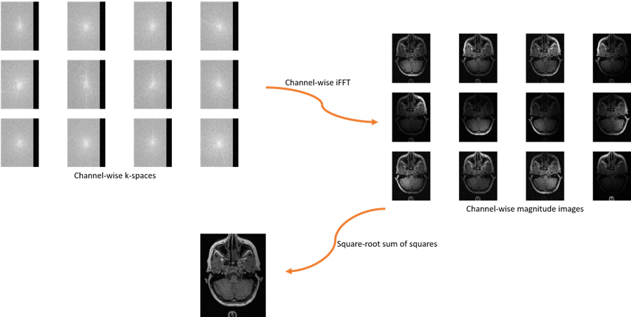
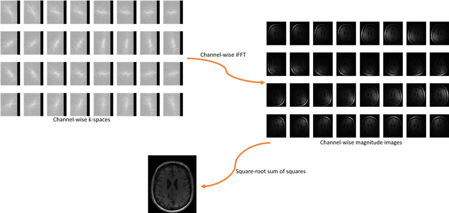
The CC dataset is composed of reconstructed images and raw k-space data of presumed normal adult subjects. The reconstructed portion of the dataset consists of 359 volumes acquired on scanners from three different vendors (GE, Philips, and Siemens) and at two magnetic field strengths (1.5 T and 3 T). Data was obtained using T1-weighted 3D imaging sequences (3D MPRAGE (Philips, Siemens), and a comparable T1-weighted spoiled gradient echo sequence (GE)) designed to produce high-quality anatomical data with 1 mm3 voxels. Further information and sample images are provided in Table 1 and Figure 1, respectively. The raw k-space portion of the dataset includes 150 3D, T1-weighted, gradient-recalled echo, sagittal acquisitions collected on a clinical MR scanner (Discovery MR750; General Electric (GE) Healthcare, Waukesha, WI). One scan corresponds to a test phantom and the remaining 149 correspond to human subjects. Datasets were acquired using either a 12-channel (112 scans) or a 32-channel coil (38 scans). Acquisition parameters were TR/TE/TI = 6.3 ms/2.6 ms/650 ms (92 scans) and TR/TE/TI = 7.4 ms/ 3.1 ms/400 ms (58 scans), with 170 to 180 contiguous 1.0-mm thick slices and a field of view of 256 mm × 218 mm. The acquisition matrix size for each channel was Nx×Ny×Nz = 256×218×[170,180]. In the slice-encoded direction (kz), data were partially collected up to Nz=[145,160] and then zero filled to Nz=[170,180]. The scanner automatically applied the inverse Fourier Transform, using the fast Fourier transform (FFT) algorithms, to the kx-ky-kz k-space data in the frequency-encoded direction, so a hybrid x-ky-kz dataset was saved. This reduces the problem from 3D to two-dimensions, while still allowing under-sampling of k-space in the phase-encoding (ky) and slice-encoding directions (kz). The partial Fourier reference data were reconstructed by taking the channel-wise iFFT of the collected k-spaces for each slice of the 3D volume and combining the outputs through the conventional square root sum of squares algorithm.18 No warping correction was applied. Sample 12-channel and 32-channel are depicted in Figures 2 and 3, respectively. The raw k-space dataset is split into train, validation and test sets (see Table 2). Only the train and validation sets composed of 12-channel data are currently public. Research teams can use these data and the reconstructed images to develop their MR reconstruction algorithms and submit their models for assessment in the test set. The metrics used to assess reconstruction are reconstruction time using standardized hardware, peak signal to noise ratio (pSNR), normalized root mean squared error (nRMSE), and visual information fidelity (VIF).19 VIF recently has been shown to have a strong correlation with the radiologist assessment of image quality.Results
The entire dataset provides > 200 GB of presumed normative brain MR data. The average acquisition time for the fully sampled version of our 3D raw k-space data was 341 seconds. The average age of our subjects was 44.5 years ± 15.5 years (mean ± standard deviation) with a range from 20 years to 80 years. Unlike fastMRI, our data correspond to three-dimensional (3D) acquisitions, which are theoretically sparser compared to two-dimensional (2D) acquisitions. The CC dataset has had 220 downloads coming from over 50 different research institutions (6 Nov 2019) and it is currently hosting an ongoing online MR reconstruction challenge that will remain open until after May 2020.Discussion
The CC data allow development and assessment of MR reconstruction algorithms. Since, our raw data corresponds to 3D acquisitions, it is possible to under-sample both in the ky and kz directions. This higher-dimensionality compared to fastMRI data allows to for greater under-sampling factors or fast acceleration factors in image acquisition. retrospectively under-sampled data can have different artifacts due to eddy current, etc. However, previous work has suggested that re-ordering the sampling to minimize gaps in k-space, these effects can be minimized.20 Finally by not (yet) making the 32-channel data publicly available and having a phantom in the test set, we expect to assess the generalizability of models that were developed with 12-channel data to 32-channel data and unseen structures (i.e., not brain).Conclusions
We proposed the CC benchmark dataset to assess MR reconstruction. The dataset is constantly being updated. In the next release, we expect to be able to provide longitudinal data that we expect can potentially be used to enhance MR reconstruction. The dataset is publicly available at https://sites.google.com/view/calgary-campinas-dataset/home.Acknowledgements
The authors would like to thank NVidia for providing a Titan V GPU, Amazon Web Services for access to cloud-based GPU services, FAPESP CEPID-BRAINN (2013/07559-3) and CAPES PVE (88881.062158/2014-01). R.S. was supported by an NSERC CREATE I3T Award and the T. Chen Fong Fellowship in Medical Imaging from the University of Calgary. R.F. holds the Hopewell Professorship of Brain Imaging at the University of Calgary. L.R. thanks CNPq (308311/2016-7).
References
1C. Qin, J. Schlemper, J. Caballero, A. N. Price, J. V. Hajnal, and D. Rueckert, “Convolutional recurrent neural networks for dynamic MR image reconstruction,” IEEE Transactions on Medical Imaging, vol. 38, no. 1, pp. 280–290, 2019.
2T. M. Quan, T. Nguyen-Duc, and W.-K. Jeong, “Compressed sensing MRI reconstruction using a generative adversarial network with a cyclic loss,” IEEE Transactions on Medical Imaging, vol. 37, no. 6, pp. 1488– 1497, 2018.
3J. Schlemper, J. Caballero, J. Hajnal, A. Price, and D. Rueckert, “A deep cascade of convolutional neural networks for dynamic MR image reconstruction,” IEEE Transactions on Medical Imaging, vol. 37, no. 2, pp. 491–503, 2018.
4L. Xiang, Y. Chen, W. Chang, Y. Zhan, W. Lin, Q. Wang, and D. Shen, “Deep learning based multi-modal fusion for fast MR reconstruction,” IEEE Transactions on Biomedical Engineering, 2018.
5G. Yang, S. Yu, H. Dong, G. Slabaugh, P. L. Dragotti, X. Ye, F. Liu, S. Arridge, J. Keegan, and Y. Guo, “DAGAN: Deep de-aliasing generative adversarial networks for fast compressed sensing MRI reconstruction,” IEEE Transactions on Medical Imaging, vol. 37, no. 6, pp. 1310–1321, 2018.
6P. Zhang, F. Wang, W. Xu, and Y. Li, “Multi-channel generative adversarial network for parallel magnetic resonance image reconstruction in k-space,” in International Conference on Medical Image Computing and Computer-Assisted Intervention (MICCAI). Springer, 2018, pp. 180–188.
7B. Zhu, J. Z. Liu, S. F. Cauley, B. R. Rosen, and M. S. Rosen, “Image reconstruction by domain-transform manifold learning,” Nature, vol. 555, no. 7697, p. 487, 2018.
8T. Eo, Y. Jun, T. Kim, J. Jang, H.-J. Lee, and D. Hwang, “Kiki-net: crossdomain convolutional neural networks for reconstructing undersampled magnetic resonance images,” Magnetic Resonance in Medicine, vol. 80, no. 5, pp. 2188–2201, 2018.
9J. Sun, H. Li, Z. Xu et al., “Deep ADMM-net for compressive sensing MRI,” in Advances in Neural Information Processing Systems, 2016, pp. 10–18.
10S. Wang, Z. Su, L. Ying, X. Peng, S. Zhu, F. Liang, D. Feng, and D. Liang, “Accelerating magnetic resonance imaging via deep learning,” in IEEE International Symposium on Biomedical Imaging (ISBI). IEEE, 2016, pp. 514–517.
11K. Hammernik, T. Klatzer, E. Kobler, M. P. Recht, D. K. Sodickson, T. Pock, and F. Knoll, “Learning a variational network for reconstruction of accelerated MRI data,” Magnetic Resonance in Medicine, vol. 79, no. 6, pp. 3055–3071, 2018.
12Y. Han, J. Yoo, H. Kim, H. Shin, K. Sung, and J. Ye, “Deep learning with domain adaptation for accelerated projection-reconstruction MR,” Magnetic resonance in medicine, vol. 80, no. 3, pp. 1189–1205, 2018.
13K. Zeng, Y. Yang, G. Xiao, and Z. Chen, “A very deep densely connected network for compressed sensing mri,” IEEE Access, vol. 7, pp. 85 430– 85 439, 2019.
14M. Mardani, E. Gong, J. Y. Cheng, S. S. Vasanawala, G. Zaharchuk, L. Xing, and J. M. Pauly, “Deep generative adversarial neural networks for compressive sensing MRI,” IEEE Transactions on Medical Imaging, vol. 38, no. 1, pp. 167–179, 2019.
15R. Souza, R. M. Lebel, and R. Frayne, “A hybrid, dual domain, cascade of convolutional neural networks for magnetic resonance image reconstruction,” in Proceedings of The 2nd International Conference on Medical Imaging with Deep Learning, ser. Proceedings of Machine Learning Research, vol. 102. London, United Kingdom: PMLR, 08–10 Jul 2019, pp. 437–446.
16J. Zbontar, F. Knoll, A. Sriram, M. J. Muckley, M. Bruno, A. Defazio, M. Parente, K. J. Geras, J. Katsnelson, H. Chandarana et al., “fastMRI: An open dataset and benchmarks for accelerated MRI,” arXiv preprint arXiv:1811.08839, 2018.
17R. Souza, O. Lucena, J. Garrafa, D. Gobbi, M. Saluzzi, S. Appenzeller, L. Rittner, R. Frayne, and R. Lotufo, “An open, multi-vendor, multifield-strength brain MR dataset and analysis of publicly available skull stripping methods agreement,” NeuroImage, 2017.
18E. G. Larsson, D. Erdogmus, R. Yan, J. C. Principe, and J. R. Fitzsimmons, “Snr-optimality of sum-of-squares reconstruction for phased-array magnetic resonance imaging,” Journal of Magnetic Resonance, vol. 163, no. 1, pp. 121–123, 2003.
19A. Mason, J. Rioux, S. Clarke, A. Costa, M. Schmidt, V. Keough, T. Huynh, and S. Beyea, “Comparison of objective image quality metrics to expert radiologists’ scoring of diagnostic quality of MR images.” IEEE transactions on medical imaging, 2019.
20MER Jones, R Frayne, RM Lebel. Image quality impact of randomized sampling trajectories: implications for compressed sensing and a correction strategy Image quality impact of randomized sampling trajectories: implications for compressed sensing and a correction strategy. International Society of Magnetic Resonance in Medicine Annual Meeting, 22-27 April 2017, Honolulu, Hawaii, USA
Figures