3585
Untrained Modified Deep Decoder for Joint Denoising and Parallel Imaging Reconstruction
Sukrit Arora1, Volkert Roeloffs1, and Michael Lustig1
1UC Berkeley, Berkeley, CA, United States
1UC Berkeley, Berkeley, CA, United States
Synopsis
An untrained deep learning model based on a Deep Decoder was used for image denoising and parallel imaging reconstruction. The flexibility of the modified Deep Decoder to output multiple images was exploited to jointly denoise images from adjacent slices and to reconstruct multi-coil data without pre-determed coil sensitivity profiles. Higher PSNR values were achieved compared to the traditional methods of denoising (BM3D) and image reconstruction (Compressed Sensing). This untrained method is particularly attractive in scenarios where access to training data is limited, and provides a possible alternative to conventional sparsity-based image priors.
Introduction
Trained reconstruction networks such as Variational Networks1 and Deep Convolutional Neural Networks2 outperform traditional, non-learning based methods in tasks such as MR image denoising and reconstruction. However, their success depends on access to large training datasets and ground truth data. In the clinical context, the small amount of available training data and the lack of ground-truth data may make training-based techniques difficult to apply in practice. Recently, Ulyanov and coworkers proposed a method3 that solves inverse problems without any training data, observing that the network architecture itself serves as a prior biased toward "natural" images.This idea of an untrained network as a prior is then expounded on by Heckel, who presents a simpler yet improved network architecture called a Deep Decoder4,5 (DD).In this work, we modify the DD and investigate its use to perform two different tasks without training: multi-slice denoising and parallel imaging reconstruction.
Theory
The DD architecture (Figure 1) is a generative decoder model that starts with a fixed, randomly-generated tensor $$$z$$$, and generates $$$k_{\text{out}}$$$ output images through pixel-wise linear combinations of channels, ReLU non-linearities, channel normalizations, and bilinear interpolation upsampling. Specifically, at every layer, the network performs the following operation: $$T_{l+1}=U_l\text{cn}(\text{relu}(T_lC_l))~\forall l\in \{0, \dots, d-1\}$$ where $$$T_l$$$ is the tensor at layer $$$l$$$ ($$$T_0=z$$$) and $$$C_l \in \mathcal{R}^{k\times k}$$$ are the weights of the network at layer $$$l$$$. The expression $$$T_lC_l$$$ is a linear combination of $$$T_l$$$ across all channels. The $$$U_l$$$ is the bilinear upsampling operator which upsamples the spatial dimensions from $$$(h_l,w_l)$$$ to $$$(h_{l+1},w_{l+1})$$$. Finally, the output of the network $$$G_w(z)$$$ is formed by $$$G_w(z)=T_dC_d$$$, where $$$C_d \in \mathcal{R}^{k \times k_{\text{out}}}$$$.Methods
The original DD network is modified in three ways: First, non-integer upsampling factors between layers were implemented to enable arbitrary output dimensions; second, the sigmoid in the final layer was removed to support an unconstrained output range; and third, the output channels of the network were identified with either multiple slices (denoising) or multiple channels (image reconstruction).This modified DD (mDD) is then used to solve inverse problems by minimizing the objective function $$f(w)=||AG_w(z)-y||^2_2$$ with respect to the weights $$$w$$$ for a single observation $$$y$$$ and a given forward model $$$A$$$. For denoising, we set $$$A=I$$$, and identify the network output channels with the set of slices to be jointly denoised. For multi-coil image reconstruction, we set $$$A=P_k\mathcal{F}$$$, where $$$P_k$$$ is the k-space subsampling mask and $$$\mathcal{F}$$$ is the Fourier Transform. Here, we identify the network output channels with the individual coil images (so no predetermined sensitivity maps are necessary).
Our PyTorch implementation is based on the original DD implementation4 and uses the ADAM optimizer6 (learning rate of 0.01). Depending on the number of parameters of the network, the number of iterations was 5,000 when overparameterized (early stopping) or 50,000 when underparameterized (running to convergence). Complex data is processed by representing real and imaginary parts separately in the channel dimensions of the network.
For reference, we used single-slice mDD and BM3D7 to compare denoising, and parallel imaging / compressed sensing (CS) to compare reconstruction8.
Results
Figure 2 shows the effect of jointly denoising 10 adjacent slices of a synthetic data set (BrainWeb9). Joint denoising outperforms both BM3D denoising and single-slice mDD denoising and results in a maximal pSNR improvement of 1.54 dB. BM3D leaves some blocky artifacts, giving a pixelated appearance, while the single-slice mDD instead blurs some of the details. Joint denoising preserves structure better at a reduced artifact level.Figure 3 shows a 4x and 8x accelerated parallel imaging reconstruction of acquired 15 channel knee data from the FastMRI NYU dataset10. Similar to its denoising performance, the mDD performs better than CS with a maximal pSNR improvement of 1.39 dB in the 4x case and 2.58 dB in the 8x case.
Discussion and Conclusion
Our results show that joint denoising preserves structure better and reduces the artifact level compared to individually optimizing with the mDD.For parallel imaging, the mDD generates images with a reduced level of aliasing artifacts. We hypothesize that the network output is biased toward smooth, unaliased images.
The results show that the Modified Deep Decoder architecture allows a concise representation of MR images. The flexibility of this generative image model was successfully leveraged to jointly denoise adjacent slices in 3D MR images and to reconstruct multi-coil data without explicit estimation of coil sensitivities.
This untrained method is particularly attractive in scenarios when access to training data is limited and provides a possible alternative to conventional sparsity-based image priors.
Acknowledgements
References
- Hammernik, Kerstin et al. “Learning a Variational Network for Reconstruction of Accelerated MRI Data.” Magnetic Resonance in Medicine 79.6 (2018): 3055–3071. Magnetic Resonance in Medicine. Web.
- Sandino, Christopher M, and Joseph Y Cheng. “Deep Convolutional Neural Networks for Accelerated Dynamic Magnetic Resonance Imaging.” Stanford University CS231N, Course project (2017): n. pag. Stanford University CS231N, Course project. Web.
- Ulyanov, Dmitry, Andrea Vedaldi, and Victor Lempitsky. “Deep Image Prior Journel.” The IEEE Conference on Computer Vision and Pattern Recognition (CVPR) (2018): n. pag. Print.
- Heckel, Reinhard, and Paul Hand. “Deep Decoder: Concise Image Representations from Untrained Non-Convolutional Networks.” (2018): n. pag. Web.
- Heckel, Reinhard. “Regularizing Linear Inverse Problems with Convolutional Neural Networks.” (2019): n. pag. Web.
- Kingma, Diederik P. and Ba, Jimmy Adam: A Method for Stochastic Optimization. (2014). , cite arxiv:1412.6980Comment: Published as a conference paper at the 3rd International Conference for Learning Representations, San Diego, 2015.
- K. Dabov, A. Foi, V. Katkovnik, and K. Egiazarian, “Image denoising with block-matching and 3D filtering,” Proc. SPIE Electronic Imaging '06, no. 6064A-30, San Jose, California, USA, January 2006.
- Lustig, Michael et al. “Compressed Sensing MRI: A Look at How CS Can Improve on Current Imaging Techniques.” IEEE Signal Processing Magazine 2008: 72–82. IEEE Signal Processing Magazine. Web.
- C.A. Cocosco, V. Kollokian, R.K.-S. Kwan, A.C. Evans : "BrainWeb: Online Interface to a 3D MRI Simulated Brain Database" NeuroImage, vol.5, no.4, part 2/4, S425, 1997 -- Proceedings of 3-rd International Conference on Functional Mapping of the Human Brain, Copenhagen, May 1997.
- Zbontar, Jure et al. “FastMRI: An Open Dataset and Benchmarks for Accelerated MRI.” (2018): n. pag. Web.
Figures
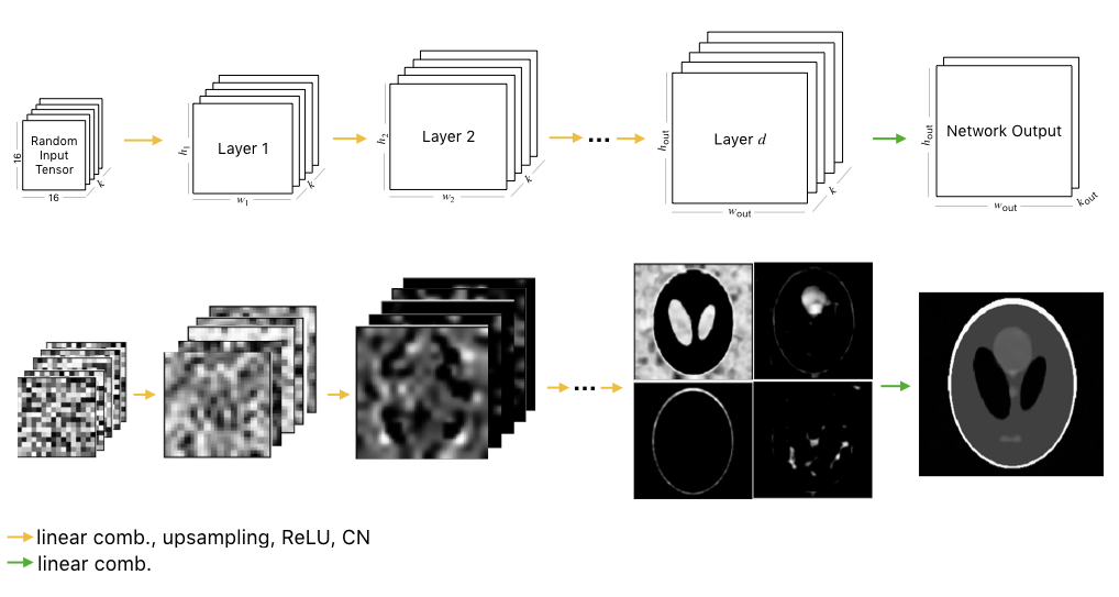
Figure 1: (Top) Deep Decoder network architecture visualized. (Bottom) Activation maps for network visualized for a Shepp-Logan phantom for $$$k=64$$$ and $$$k_{\text{out}}=1$$$. Selected channels illustrate data flow.
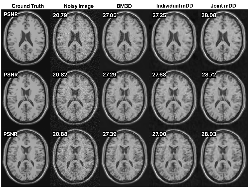
Figure 2: Selected 3 out of 10 adjacent slices denoised using BM3D, single-slice denoising ($$$k=64$$$, $$$k_{\text{out}}=1$$$) mDD, and joint denoising ($$$k=64$$$, $$$k_{\text{out}}=10$$$) mDD where the network denoises all 10 slices simultaneously. The number of parameters up to the output layer are the same in both the slice-wise and joint mDD method.
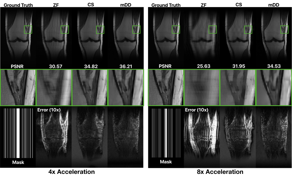
Figure 3: Reconstruction of subsampled k-space data with acceleration factors of 4 and 8 respectively. For each acceleration factor, the reconstructions are (from left to right) 1. zero filled (ZF), 2. Compressed Sensing (CS), and 3. mDD, with $$$k=256$$$ and $$$k_{\text{out}}=30$$$ (complex data). Center row is a zoomed-in region. The bottom row shows the subsampling mask and error maps.