3583
Reconstruction of Quantitative Susceptibility Maps from the Phase of Susceptibility-Weighted Images Using a Deep Neural Network1Center for Brain Imaging Science and Technology, Department of Biomedical Engineering, Key Laboratory for Biomedical Engineering of Ministry of Education, Zhejiang University, Hangzhou, China, 2MR Collaboration, Siemens Healthcare Ltd, Shanghai, China, 3Department of Imaging Sciences, University of Rochester, Rochester, NY, United States
Synopsis
There is a need to obtain quantitative measures of tissue susceptibility in the form of susceptibility-weighted imaging (SWI). In this study, we used a deep neural network to generate QSM maps from SWI high pass (HP)–filtered phase images. Using the QSM maps reconstructed from mGRE data by iLSQR (mGRE iLSQR) as the ground truth, the QSM maps generated from SWI HP-filtered phase images by UNet (SWI UNet) resulted in lower residuals and a better performance in quantitative metrics compared with the QSM maps reconstructed from SWI HP-filtered phase images by iLSQR (SWI iLSQR).
Introduction
Quantitative susceptibility mapping (QSM) is a growing field of research in MRI, aimed at noninvasively estimating the magnetic susceptibility of biological tissue 1,2. However, using multi-echo gradient-recalled echo (mGRE) for QSM requires long scan and reconstruction times, and mGRE is not widely applied in clinical use. Susceptibility-weighted imaging (SWI) has been widely applied to diagnose various venous abnormalities and image a range of pathologies 3. SWI uses a three-dimensional (3D) gradient-recalled echo (GRE) scan, and four sets of images were generated: the original magnitude, HP-filtered phase, susceptibility-weighted, and mIPs over the susceptibility-weighted images. However, SWI cannot directly provide quantitative measures of magnetic susceptibility, even though the HP-filtered phase data of SWI contain susceptibility information. The phase data of SWI are HP-filtered, which removes the background phase, but also removes a substantial portion of low-frequency components of the tissue phase, so the susceptibility quantification will be inaccurate 4. Recently, a UNet-based convolutional neural network has been successfully used to generate susceptibility source maps from the phase data of a GRE sequence 5,6. In this study, we developed a deep neural network pipeline to generate QSM maps from SWI HP-filtered phase images.Methods
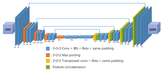
Nine healthy volunteers were recruited, and MR data were acquired on a 3T scanner (MAGNETOM Prisma, Siemens Healthcare, Erlangen, Germany) using a 20-channel head-neck coil with the following sequences: (1) SWI: TR = 28 ms, TE = 20 ms, flip angle = 15o, voxel size = 1.1*1.1*1.6 mm3, readout bandwidth = 120 Hz/pixel, with a scan time of 3 min 38 s. (2) mGRE: 8-echo readout, TR = 53 ms, TE1 = 3.63 ms, echo spacing (ESP) = 5.1 ms, flip angle = 20o, voxel size = 1.1*1.1*1.6 mm3, readout bandwidth = 300 Hz/pixel, with a scan time of 16 min 18 s.For training, the labeling data we used included QSM maps reconstructed from mGRE data with an improved least-squares (iLSQR) method 7. The deep neural network we used is shown in Figure 1, with the UNet 8 structure modified from 2D to 3D to take 3D inputs and generate 3D outputs, so that a 3D SWI HP-filtered phase image was taken as an input and the same size 3D QSM images were generated. Data from eight randomly selected subjects were used as training data, and data from the remaining subject were used as the testing data. To augment the training data, we tripled the information by rotating the data 90o and horizontally flipping the data. We ultimately obtained 6778 training patches with a size of 48*48*48 pixels.
After training, the testing data were applied to the trained 3D UNet to generate QSM maps. Three error metrics 9, root-mean-square error (RMSE), high-frequency error norm (HFEN), and structural similarity index (SSIM), were used to measure the quality of the QSM maps reconstructed from SWI HP phase data by the neural network and iLSQR. In addition, we performed a comparison analysis in selected region of interests (ROIs).
Results
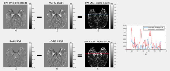
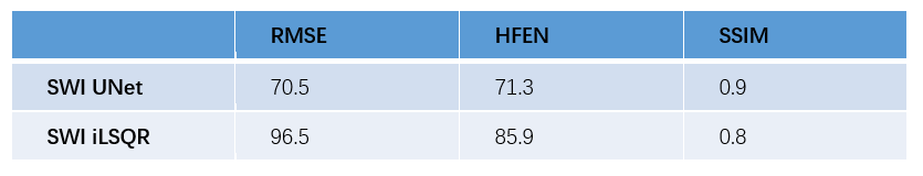
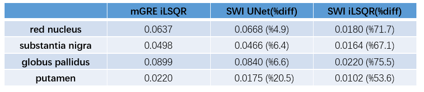
As shown in Figure 2, we compared the QSM maps reconstructed from the SWI HP-filtered phase data by 3D UNet and iLSQR. The SWI UNet result was more similar to the ground truth, with lower residuals. In Table 1, we show the quantitative metrics of SWI UNet and SWI iLSQR. The network results had a lower RMSE, lower HFEN, and higher SSIM. The outcome of the ROI analysis is shown in Table 2, and the results of the neural network were shown to be much closer to those of the ground truth in selected ROIs.Discussion and Conclusion
In this work, we used a 3D UNet to reconstruct QSM maps by using SWI HP-filtered phase images. The 3D UNet results were more similar to the ground truth with lower residuals and performed better in quantitative metrics than QSM maps generated from the SWI HP-filtered phase images by the traditional method. However, there remained some artifacts in the neural network results and the results were smooth in some tissues. The method may be improved by using more training subjects and optimized deep neural networks.Acknowledgements
This work was supported by the National Natural Science Foundation of China [grant numbers 91632109, 81871428, 81971184], the Shanghai Key Laboratory of Psychotic Disorders [grant number 13dz2260500], the Major Scientific Project of Zhejiang Lab [grant number 2018DG0ZX01], and the Fundamental Research Funds for the Central Universities [grant number 2019QNA5026].References
1.Wang Y, Liu T. Quantitative susceptibility mapping (QSM): Decoding MRI data for a tissue magnetic biomarker. Magn Reson Med 2015; 73:82–101.
2.Deistung A, Schweser F, Reichenbach JR. Overview of quantitative susceptibility mapping. NMR Biomed 2017;30:e3569.
3.Haacke EM, Xu Y, Cheng YC, Reichenbach JR. Susceptibility weighted imaging (SWI). Magn Reson Med 2004;52:612–618
4.Liu C, Li W, Tong KA, Yeom KW, Kuzminski S. Susceptibility-weighted imaging and quantitative susceptibility mapping in the brain. J. Magn. Reson. Imaging 2015; 42(1): 23–41.
5.Yoon J, Gong E, Chatnuntawech I, Bilgic B, Lee J, Jung W, et al. Quantitative susceptibility mapping using deep neural network: QSMnet. Neuroimage 2018;179:199–206.
6.Rasmussen KGB, Kristensen MJ, Blendal RG, Ostergaard LR, Plocharski M, O’Brien K, et al. Deep QSM-using deep learning to solve the dipole inversion for MRI susceptibility mapping. Biorxiv 2018:278036.
7.Li W, Wang N, Yu F, Han H, Cao W, Romero R, Tantiwongkosi B, Duong TQ, Liu C. A method for estimating and removing streaking artifacts in quantitative susceptibility mapping. Neuroimage. 2015;108:111–22
8.Ronneberger O, Fischer P, Brox T. U-net: Convolutional networks for biomedical image segmentation. Medical image computing and computer-assisted intervention – MICCAI 9351 (2015): 234-241.
9.Langkammer, C., Schweser, F., Shmueli, K., Kames, C., Li, X., Guo, L., Milovic, C., Kim, J., Wei, H., Bredies, K., Buch, S., Guo, Y., Liu, Z., Meineke, J., Rauscher, A., Marques, J.P., Bilgic, B. Quantitative susceptibility mapping: report from the 2016 reconstruction challenge. Magn. Reson. Med. 79, 1661–1673.
Figures