Introduction

The RF safety assessment of metallic implants is a computationally demanding task. Therefore, an alternative sparse inverse computation approach was presented.¹ The problem is that the time complexity of this method scales poorly with the problem size, $N$. For direct matrix inversion,$$$\,\mathcal{O}(N^3)$$$, or$$$\,\mathcal{O}(\sqrt{k}N)\,$$$for a conjugate gradient method. Where$$$k$$$is the condition number, which for realistic problems is in the order of$$$\,10^6-10^8$$$. Recently, deep learning unrolled optimization approaches have been published that drastically decrease the number of iterations required to find the solution to the inverse formulation.^2,3,4 In this work, we use such an approach to further reduce the computation time of the local field enhancement near implants.

Theory

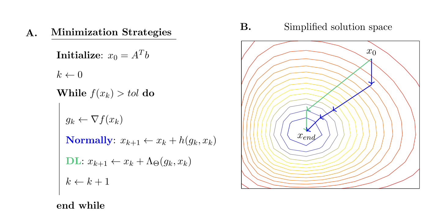
The RF field perturbation due to a metallic implant with respect to an incident RF field can be obtained in an efficient manner through a matrix inversion on a relatively small domain,^1,5$$f^{tot}=f^{inc}+Z\left(I-\Delta{C}S^TZ\right)^{-1}\Delta{C}S^Tf^{inc}.$$Here $$$f^{tot}$$$ contains the total electromagnetic fields, whereas$$$\,f^{inc}\,$$$contains the incident fields. Further,$$$\,Z\,$$$is a library matrix that consists of the single point source field responses for each location defined by$$$\,S\,$$$. At these locations a change in electromagnetic properties ($$$\Delta{C}$$$) is possible. Finally,$$$\,I\,$$$is the identity matrix.
The solution to Equation (1) (which is equivalent to the scattered current density on the implant) can be found by solving,$$\min_{x}\frac{1}{2}||Ax-b||_n^2,$$in an iterative fashion, for a given norm$$$\,n\,$$$. Various minimization strategies exist to solve this problem but these are not tailored specifically to the class of problems at hand and can, therefore, be considered suboptimal. Recently, neural networks have been introduced into these minimization problems.^2,3,4 The algorithm shown in Figure 1A tries to minimize$$$\,f=\frac{1}{2}||Ax-b||_2^2\,$$$. Here $$$\Lambda_{\Theta}$$$ can be any neural network where the iterations that are required to find the solution to the problem are rolled out into all the separate layers of a neural network. This can be seen as,$$\Lambda_{\Theta}=(\mathcal{A}_k\circ\mathcal{M}_{w_k,b_k})\circ(\mathcal{A}_{k-1}\circ\mathcal{M}_{w_{k-1},b_{k-1}})\circ\cdots\circ(\mathcal{A}_1\circ\mathcal{M}_{w_1,b_1}),$$where$$$\,\mathcal{A}\,$$$and $$$\,\mathcal{M}\,$$$are nonlinear and affine operators respectively with the learnable parameters,$$$\,\Theta\,$$$, given by,$$\Theta=\left((w_k,b_k),(w_{k-1},b_{k-1}),\cdots,(w_1,b_1)\right).$$Either all the parameters of the network are learned at once or a greedy learning approach can be taken which only trains one iteration, to a specified accuracy, at a time.² This allows the gradient computation to be taken outside of the training which saves considerable time and memory. Finally, if after $$$\,k\,$$$ iterations the residual of the costfunctional is too large, one can train a$$$\,(k+1)^{\text{th}}\,$$$iterate or solve the problem with the traditional method with a very good initial guess (a hybrid method). Once finished the network has learned the solution space (Figure 1B) of the problem at hand, i.e. electromagnetic inversion, and can find the solution to new problems very efficiently.

Methods

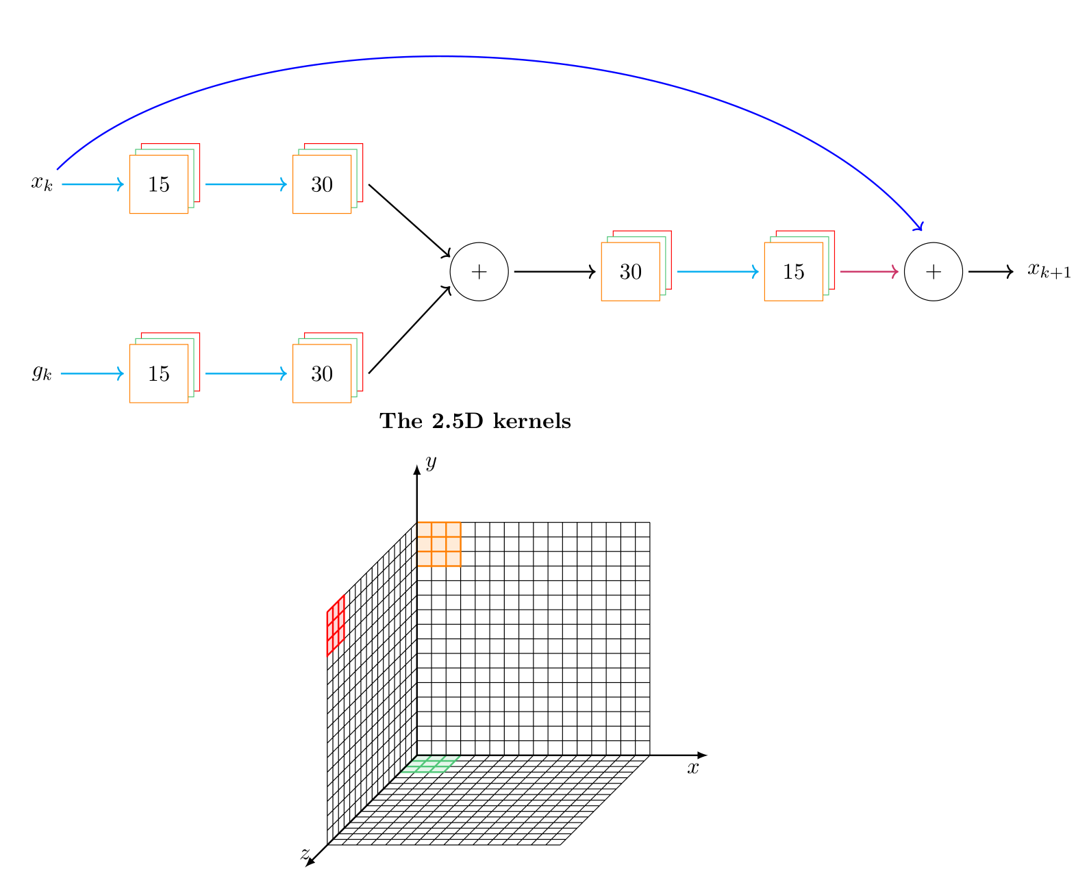
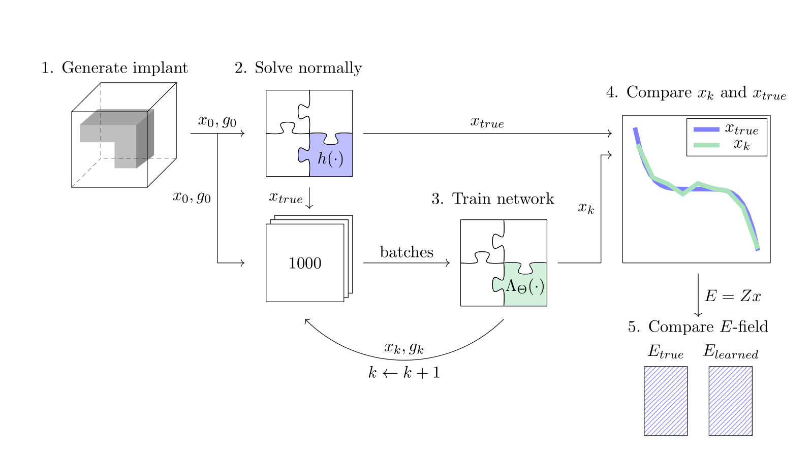
The network architecture for a single iteration can be seen in Figure 2. For training the network the training and test sets were generated using the traditional minimization strategy. In total 10.000 random implants are generated, for which the initial guess ($$$x_0=A^Tb$$$) and the corresponding gradient are computed. The training set consists of 95% of the data, the remaining data were used for the test set. The library used is one computed within the brain of Duke. In total 5 iterations were trained, where between iterations the new gradient for each problem was computed to make the training data for the following iteration. The entire pipeline, as seen in Figure 3, is programmed in the Julia language,⁶ where the deep learning framework Flux.jl is used. The evaluation is based on the found solution with the learned iterations and the found electric field using the hybrid method, i.e. first using the learned iterations and using that as an initial guess for the traditional minimization strategy.

Results

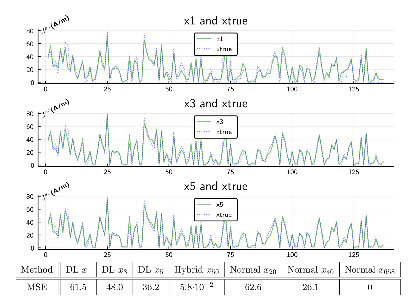
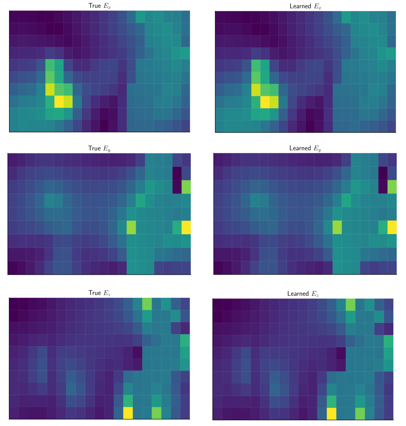
In Figure 4 an 8 times undersampled output of the network's solution is shown compared to the true solution. In the table at the bottom, it can be observed that the Mean Squared Error (MSE) of the deep learned approach decreases much faster compared to the normal one. The Hybrid method finds a numerically equivalent solution in 13 times fewer iterations (i.e. 13 times faster). The resulting electric field is shown in Figure 5.

Discussion

The deep learning approach to solve the inverse problem greatly reduces the computation time. For the implants shown in [1], this would be 0.1 to 1s computation time. Furthermore, the training of the network requires fewer data compared to other neural networks since it only learns a very small part of the problem: the computation of the step size and direction. The underlying physical model is still present in this methodology creating more confidence in the obtained solution. Finally, the ability to use the proposed approach in conjunction with the normal solving strategy results in a fast and reliable method for RF safety assessment of implants. The proposed methodology represents an important next step towards TIER 4 safety analysis or even online RF safety assessment for implants. The latter would enable patients with non-labeled implants to undergo an MRI-exam.

Conclusion

The deep learning approach to solve inverse electromagnetic problems greatly reduces the number of iterations required to find the solution. This work poses the next step towards online RF safety assessment of implants. Furthermore, the combination with the traditional minimization allows for both large acceleration and high accuracy for the local RF field enhancement due to implants.

Acknowledgements

The authors would like to thank both Niek Huttinga and Janot Tokaya for interesting discussions.