Introduction

Simultaneous proton (¹H) and sodium (²³Na) acquisition can provide important metabolic information¹. To obtain sufficient SNR for ²³Na, a center outward (CO) radial trajectory with a long dwell time (small acquisition bandwidth) is desired². Unfortunately, such sampling strategies generally lead to blurred ¹H images due to the larger gyromagnetic ratio of ¹H compared to ²³Na. Therefore, ¹H images need to be corrected for off-resonance effects. In this work we train a convolutional neural network (CNN) that performs an off-resonance correction without an additional measured field map. Instead, we use two images as inputs: the usual CO image, and an image obtained from a center-inward (CI) trajectory captured during the rephase gradient. Such images are acquired with different effective TE and acquisition windows, and hence encode the field map without increasing scan time.

Methods

Training data: 70 MP-RAGE and 63 T₂-weighted 3D brain images from the Human Connectome Project (https://ida.loni.usc.edu/login.jsp) were downloaded and transformed into transverse (MPRAGE:40, T₂w:65) and sagittal (MPRAGE:36, T₂w:66) slices. The slices for one MP-RAGE and one T₂-weighted volunteer were selected to create a model validation set.
Simulation: Linear, uniform and Gaussian-shaped ΔB₀ maps with a maximum absolute off-resonance value of 500 Hz were simulated. Each 2D image was blurred for the CO (4.8 ms) and the CI (1 ms) trajectories, using one of the simulated ΔB₀ maps and a TE of 1.5 ms. After blurring, data were augmented by rotating each image by multiples of 90 degrees, resulting in 26,580 training and 828 validation examples. A Gaussian-shaped phase offset was randomly added for each CO/CI pair. Images were normalized (absolute values between 0 and 1), and real and imaginary image components for the CO and the CI trajectories were used as 4-channel input. One Gaussian-shaped ΔB₀ map was shifted by ~100 Hz and used to simulate an additional validation example.
Model and training: We used a residual neural network with three residual blocks containing two layers each³. A 2D convolution using 3×3 kernels and 128 features was performed at every layer. ReLu (hidden layers) and tanh (output layer) activations were used. We minimized the mean absolute error over 6 epochs using the Adam optimizer with an initial learning rate of 5x10^-4 and a batch size of 16. Drop out with a probability of 0.25 was applied to all the layers except the last one. Training was performed in Tensorflow with a GeForce RTx 2060 gpu.
Test data acquisition: Blurred CO and CI images were acquired using a 7T MR system (MAGNETOM, Siemens, Erlangen, Germany) with a 32 channel Nova head coil for phantom experiments and an 8-channel dual tune coil for in vivo brain experiments (informed consent obtained). Each scan was performed using 1) B₀ shimming, 2) intentionally perturbed shim settings, and 3) with a constant offset of 300 Hz to the scanner’s resonance frequency. Scan parameters: 1x1x3 mm³ resolution, FOV=240 cm, TE/TR=1.5/10 ms, total scan time=15 s. A radial ΔB₀ map was acquired for comparison.

Results

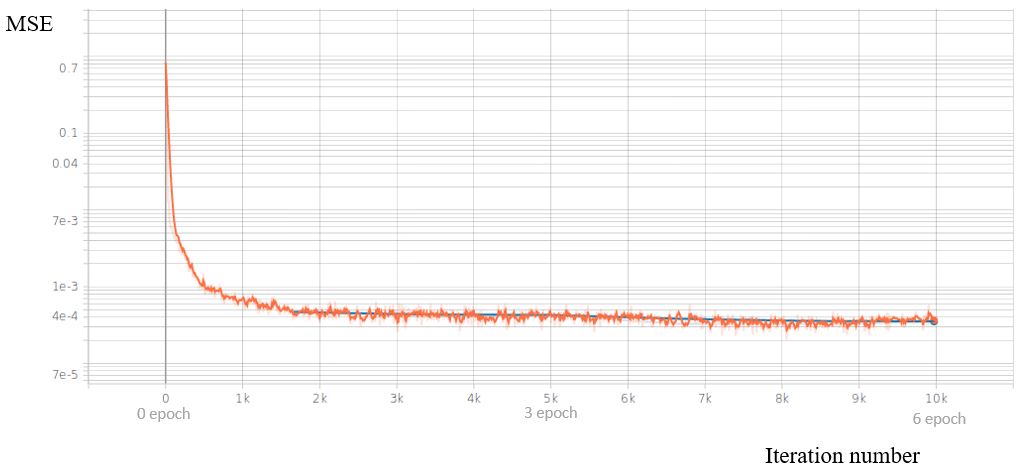
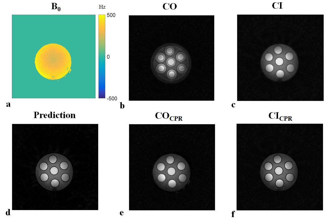
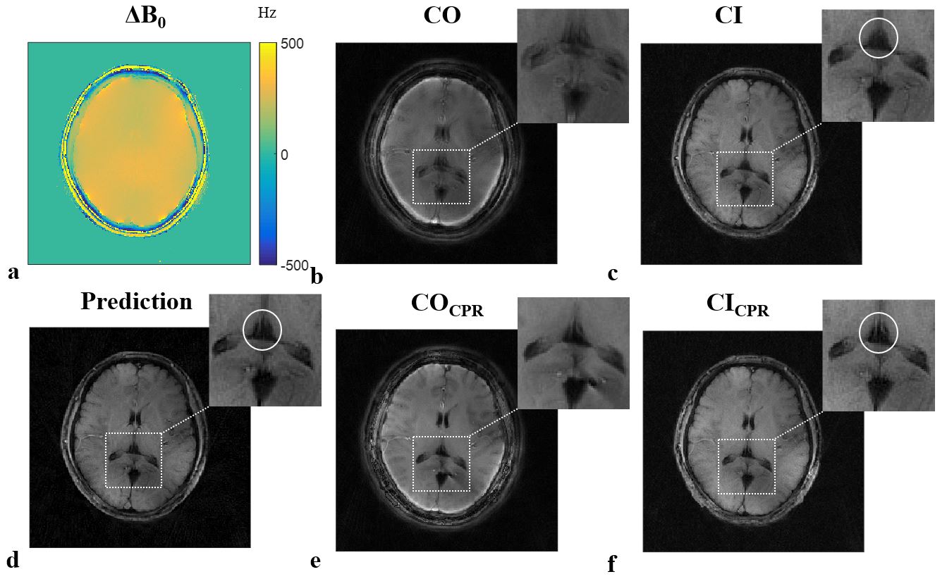
Figure 1 displays the mean squared error (MSE) loss for training and validation data during training. Figure 2 shows the deblurring performance for one slice of the validation data set. Note that the shifted Gaussian-shaped ΔB₀ map for this case did not correspond to one encountered during training. Figure 3 shows the deblurred phantom data, compared with the conjugate phase reconstruction (CPR) using the measured ΔB₀ map as input for the CO and the CI images independently. Figure 4 shows corresponding results for an in vivo brain experiment. White circles outline an example region where the prediction is sharper than both the CO and CI images. Although training of the network took 95 min, the final model corrects the blurred images in 0.19 s.

Discussion

Absolute error maps for validation data confirm that the network’s predictions are close to the ground truth images. Good performance on measured phantom data suggest that the model was not overfitted to the simulated data used for training. The trained model produces a sharper phantom image than the CPR-corrected CO image, while the trained model and CPR show similar performance for the CI phantom image. In vivo brain results also show a sharp network prediction, while CPR suffers from imperfections around the skull and loss of detail. Phantom and in vivo experiments show that, although the network predicts an image that is sharper than both the CO and the CI images, most of the contrast is learned from the CI image. This is especially visible around the fine structures in the brain image. Further optimization of the training set, for example by adapting it to the contrast of interest and by taking relaxation effects into account in simulation, may help to reduce this effect.

Conclusion

It is possible to correct for off-resonance artifacts without knowledge of the field map, using a deep learning model trained on CO and CI image pairs. This approach can be used in simultaneous radial ²³Na and ¹H acquisitions, for which a short TE and a long dwell time are necessary and CI images can be acquired efficiently. Further model optimization is necessary to improve contrast estimation around fine anatomical structures.

Acknowledgements

This project was partially funded by the Leiden University Fund (LUF) and the European Research Council Advanced Grant 670629 NOMA MRI.