Purpose

The quantitative measurement of tissue composition by MRI is conventionally challenging due to long scan time and complicated post-processing. Magnetic resonance fingerprinting (MRF) is a rapid dynamic MRI approach that aims to estimate MRI parameters in biological tissues ^1,2. The computation time of conventional MRF dictionary matching ³ becomes prohibitive for 3D acquisition or when the number of estimates increases. Deep learning is a potential alternative to dictionary matching for MRF quantification, because it can drastically reduce the computation time as demonstrated in ^4–6. This study aims to extend our newly proposed multi-layer perceptron deep learning method to achieve acceleration for MRF quantification.

Methods

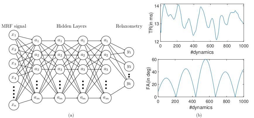
We used a 3 T human MRI scanner (Achieva TX, Philips Healthcare) with 8-channel brain and torso coils for signal reception in the brain, liver, and prostate. As shown in Figure 1, the MRF was based on an IR-FISP sequence with variable flip angles (FA) and TR ⁷. A constant speed spiral-in-spiral-out readout trajectory ⁸ with an acquisition window of 8.4 ms and acquisition factor = 58.4% was used. The trajectory was rotated by 222.5º after each dynamic. Other imaging parameters were: TR = 12.1 to 14.1 ms, FA = 0 to 60º, field-of-view = 300 × 300 mm², acquisition matrix = 256 × 256, image resolution = 1.17 × 1.17 mm², slice thickness = 5 mm, number of dynamics = 1000, number of spiral interleaves = 1. The liver MRF was scanned with 12 s breath-hold for each motion phase. Five motion phases were measured separately in five breath-holds. For a single slice brain scan, the scan time was 12 s. For a prostate MRF scan, six slices in total cost one minute to cover the entire gland. The deep neural network was based on our previous study that achieved whole-brain T1/T2 quantification in 5 s ⁹. The deep neural network contained four fully connected layers (as shown in Fig. 2 left). MRI signal evolutions from a simulated dictionary were used to train the neural network. The dictionary simulation was based on an extended phase graph algorithm that considered a constant spoiling gradient in each TR ⁷. The neural network was also trained using T1, T2, M0, simulated artifacts and varying noise levels. We also implemented a "threshold function" when training the network by giving time-courses that had L2-norm smaller than 0.8 (a.u.) background labels (i.e., zeros). Complex-valued MRF dictionary, obtained from the extended phase graph algorithm ⁷, was used for training the network. The MRF data from in vivo studies were used for testing.

Results

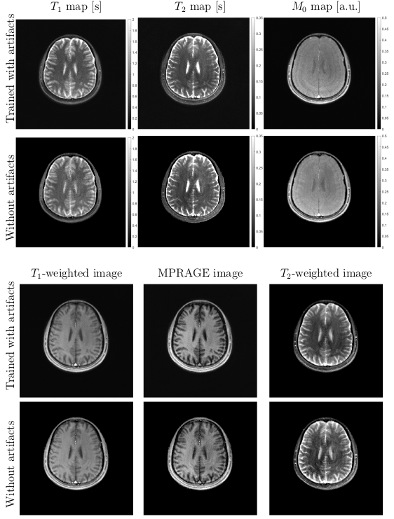
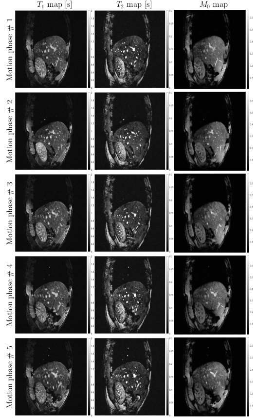
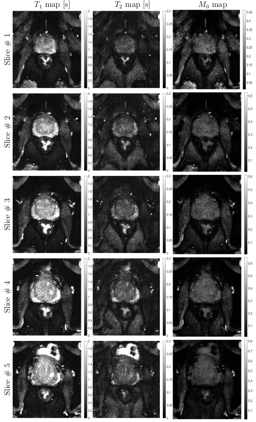
Figure 2 shows in vivo brain, liver, and prostate MRF results from the model prepared with simulated MRF artifacts and noise during training. In Figure 3, the neural network quantification of brain MRF clearly showed contrasting gray matter, white matter, and cerebrospinal fluid. The 1000 dynamics from a single slice with 256 × 256 image resolution was computed in 0.12 s. In Figure 4, liver MRF acquired from five different motion phases (one is shown), showed spatial boundaries of liver and vessels with simultaneous estimation of liver T1 and T2 at different motion phases (one is shown). The 1000 dynamics from five motion phases with 256 × 256 image resolution was computed in 0.69 s. In Figure 5, multi-slice MRF was acquired (one is shown) in a patient with prostate cancer. The T1 and T2 maps from the neural network revealed relatively clear boundaries for prostate peripheral zone, prostate central gland, obturator internus muscles, anal canal, and pubic bone. The 1000 dynamics from six slices with 256 × 256 image resolution was computed in 0.87 s.

Discussion

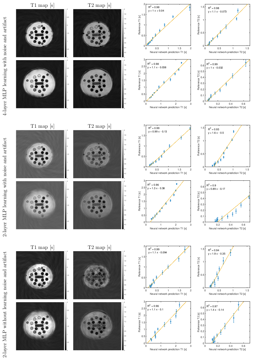
Compared with previous deep learning MRF or quantitative MRI studies ^4–6, we empirically find three key ingredients that can lead to optimal performance of the neural network under the current experimental condition, including 1) using complex-valued MRF data for quantification, 2) training the neural network with simulated MRF artifacts and noise, and 3) using four fully connected layers with sufficient representation capacity without overfitting. These three ingredients in this study had improved the estimation quality, as shown by phantom and in vivo results.

Conclusion

The proposed neural network achieved fast MRF quantification, including multi-phase and multi-slice acquisition. The model trained with simulated artifacts and noise showed reduced error in brain MRF.

References

1. Weiskopf, N. et al. Quantitative multi-parameter mapping of R1, PD(*), MT, and R2(*) at 3T: a multi-center validation. Front. Neurosci. 7, 95 (2013).
2. Latifoltojar, A. et al. Evolution of multi-parametric MRI quantitative parameters following transrectal ultrasound-guided biopsy of the prostate. Prostate Cancer Prostatic Dis. 18, 343 (2015).
3. Ma, D. et al. Magnetic resonance fingerprinting. Nature 495, 187–192 (2013).
4. Cohen, O., Zhu, B. & Rosen, M. S. MR fingerprinting Deep RecOnstruction NEtwork (DRONE). Magn. Reson. Med. 80, 885–894 (2018).
5. Balsiger, F. et al. Magnetic resonance fingerprinting reconstruction via spatiotemporal convolutional neural networks. Lect. Notes Comput. Sci. (including Subser. Lect. Notes Artif. Intell. Lect. Notes Bioinformatics) 11074 LNCS, 39–46 (2018).
6. Hoppe, E. et al. Deep learning for magnetic resonance fingerprinting: A new approach for predicting quantitative parameter values from time series. Stud. Health Technol. Inform. 243, 202–206 (2017).
7. Jiang, Y., Ma, D., Seiberlich, N., Gulani, V. & Griswold, M. A. MR fingerprinting using fast imaging with steady state precession (FISP) with spiral readout. Magn. Reson. Med. 74, 1621–1631 (2015).
8. Glover, G. H. & Law, C. S. Spiral-in/out BOLD fMRI for increased SNR and reduced susceptibility artifacts. Magn. Reson. Med. 46, 515–522 (2001).
9. Cao, P. et al. Technical Note: Simultaneous segmentation and relaxometry for MRI through multitask learning. Med. Phys. doi:10.1002/mp.13756