3568
Segmenting Tumour Habitats Using Machine Learning and Saturation Transfer Imaging
Wilfred W Lam1, Wendy Oakden1, Elham Karami1,2,3, Margaret M Koletar1, Leedan Murray1, Stanley K Liu1,2,4, Ali Sadeghi-Naini1,2,3,4, and Greg J Stanisz1,2
1Sunnybrook Research Institute, Toronto, ON, Canada, 2University of Toronto, Toronto, ON, Canada, 3York University, Toronto, ON, Canada, 4Sunnybrook Health Sciences Centre, Toronto, ON, Canada
1Sunnybrook Research Institute, Toronto, ON, Canada, 2University of Toronto, Toronto, ON, Canada, 3York University, Toronto, ON, Canada, 4Sunnybrook Health Sciences Centre, Toronto, ON, Canada
Synopsis
Saturation transfer-weighted images along with T1 and T2 maps at 7 T for 31 tumour xenografts in mice were used to automatically segment 1) tumour, 2) necrosis/apoptosis, 3) edema, and 4) muscle. Independent component analysis and Gaussian mixture modeling were used to segment these regions. Qualitatively excellent agreement was found between MRI and histopathology. An nine-image subset was identified that resulted in a 96% match in voxel labels compared to those found using the entire 24-image dataset. This subset had positive and negative predictive values of 96% and 97%, respectively, for tumour and 88% and 97%, respectively, for necrosis/apoptosis voxels.
Introduction
Intra-tumour heterogeneity is not yet considered in clinical decision-making due to the complexity of detecting and quantifying heterogeneity. Saturation transfer MRI is sensitive to tumour metabolism, microstructure, and microenvironments. This study aims to use saturation transfer: chemical exchange saturation transfer (CEST) [1] and magnetization transfer (MT) [2] to differentiate between intra-tumour regions (“habitats”), demarcate tumour boundaries, and reduce acquisition times by identifying the imaging scheme with the most impact on segmentation accuracy.Methods
Animal model:Approximately 3 × 10⁶ DU145 human prostate adenocarcinoma cells mixed in a 1:1 ratio by volume with growth factor reduced Matrigel matrix were injected in the right hind limbs of female athymic nude mice and allowed to grow into tumours (n = 31). Tumours were allowed to grow for at least 34 days post-injection to allow time for cell differentiation.
MRI and histopathology:
Saturation transfer-weighted images were acquired at 7 T over a wide range of saturation amplitudes and frequency offsets (0.5 and 2 µT between ±5 ppm and 3 and 6 µT from 300 to 3 ppm) along with T1 and T2 maps for DU145 human prostate tumour xenografts in the hind legs of nude mice (n = 31). The T1 and T2 maps were normalized by 4000 and 300 ms, respectively, which were values selected as being slightly higher than the highest values typically seen in tumour regions. After scanning, mice were sacrificed and H&E and TUNEL staining (for structural and necrosis/apoptosis information, respectively) performed.
Segmentation:
Independent component analysis (ICA; 2 components) [3] and Gaussian mixture modeling (GMM; 4 clusters) [4] were used to segment the images (Fig. 1) using five different combinations of acquired images as input ("protocols"). The weight of the first independent component (IC1) relative to the second (IC2) was also optimized. The clusters were assigned these labels: 1) tumour, 2) necrosis/apoptosis, 3) edema/subcutaneous fluid, and 4) muscle. The independent component weights and protocol giving the best qualitative match to histopathology was selected for further consideration.
The segmentation pipeline was validated by leave-one-out cross-validation for the selected protocol, where the ICA transform and GMM were trained using 30 datasets and tested on the remaining one. This validation was repeated for each mouse.
Feature selection:
In order to identify the most critical images for accurate segmentation, two- to nine-image subsets were selected by an exhaustive search that had the most voxel labels matching those of the segmentation masks generated from the full protocol. Positive and negative predictive values (PPVs and NPVs, respectively) of each subset for tumour and necrosis/apoptosis voxels were also calculated.
Results
Very good qualitative agreement was found between MRI and histopathology (first four columns in Fig. 2). The protocol with the best qualitative match to histopathology was found to be the set of 3 and 6 µT MT-weighted images and T1 and T2 maps with IC1:IC2 weights of 2:1. The segmentation masks from leave-one-out cross-validation (last column in Fig. 2) were extremely similar to those from the entire dataset except for the mouse with the large edema (last column in Fig. 2C; "mouse #3").A scatter plot of the GMM centroids is shown in Fig. 3 for segmentation using the entire data (stars) and leave-one-out (circles and crosses). The centroid groupings are consistent regardless of the training dataset except for mouse #3 (crosses). Based on correlation with histopathology, the following label assignment rules were generated. 1) The cluster with the largest absolute IC2 is labelled edema (grey). 2) Then, each dataset was reflected about the x- and y-axes as required such that the edema cluster was in the first quadrant of the Cartesian plane, since ICA does not identify the sign of the source signals. 3) Of the remaining clusters, the one with the smallest IC1 is labelled muscle (cyan); the second largest, necrosis/apoptosis (red); and the largest, tumour (blue).
The segmentation masks from the image subsets were also quite similar to those from the entire dataset (Fig. 4). A nine-image subset was identified that resulted in a 96% match in voxel labels compared to those found using the entire dataset. This subset had PPVs and NPVs of 96% and 97%, respectively, for tumour and 88% and 97%, respectively, for necrosis/apoptosis voxels. Predictive values for all the image subsets can be found in Fig. 5.
Discussion and Conclusion
Alignment and interpretation of the tissue slice compared with the MR image and segmentation mask took into consideration modifications in tissue architecture resulting from fixation, sectioning, and staining procedures. This distortion of tissue structure precluded quantitative comparisons between the segmentation masks and histopathology sections.Mouse #3 has many more edema voxels than any other tumor . Consequently, when it is left out of the training dataset, the edema centroid (grey cross in Fig. 3) shifts lower and to the left relative to all the other edema centroids (grey star and circles) and segmentation on mouse #3 fails (fifth column in Fig. 2C). This underscores the need to have a representative training dataset with sufficient numbers of voxels in each cluster.
The proposed algorithm can potentially be used to develop a robust, patient-specific tumour characterization method.
Acknowledgements
The authors thank the Canadian Institutes of Health Research (grant number PJT148660), Terry Fox Research Institute (grant number 1083), and Natural Sciences and Engineering Research Council of Canada (grant numbers CRDPJ507521-16 and RGPIN-2016-06472) for funding.References
- Ward KM, Aletras AH, Balaban RS. A New Class of Contrast Agents for MRI Based on Proton Chemical Exchange Dependent Saturation Transfer (CEST). J Magn Reson 2000;143:79–87.
- Henkelman RM, Stanisz GJ, Graham SJ. Magnetization transfer in MRI: A review. NMR Biomed 2001;14:57–64.
- Hyvärinen A, Oja E. Independent component analysis: algorithms and applications. Neural Networks 2000;13:411–430.
- Reynolds D. Gaussian Mixture Models Li, Z. S, Jain AK, editors. Encycl Biometrics 2015:827–832.
Figures
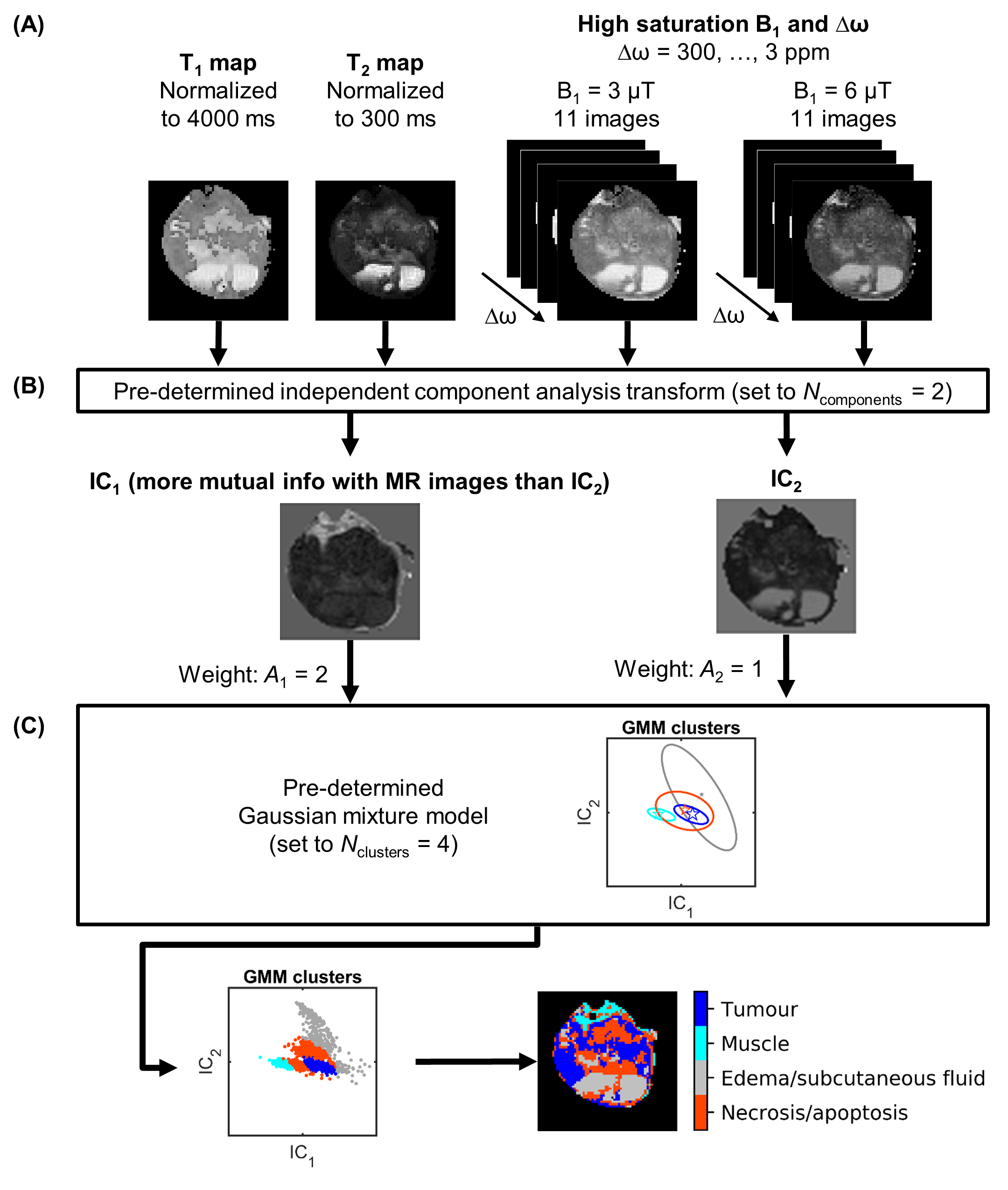
FIGURE 1. The automatic segmentation pipeline. (A) Normalized T1 and T2
maps and images acquired with various saturation B1 amplitudes
and at various frequency offsets Δω for a representative
mouse. (B) Non-background voxels were transformed by a pre-determined independent component analysis transform, which was set to
generate two independent components (ICs). (C) The ICs were then input to a pre-determined Gaussian mixture model, which was set to 4 clusters, and clusters were assigned labels.
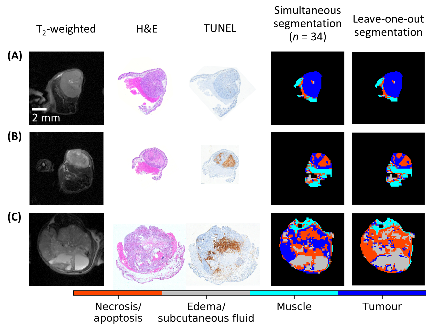
FIGURE 2. Comparison of whole-dataset and
leave-one-out segmentation with anatomical images and histology. In all cases, the brown
areas indicating necrosis/apoptosis in the TUNEL sections (third column) match
well with the red areas of the whole-dataset segmentation
masks (fourth column). Variance from the histology is seen with the leave-one-out segmentation masks
(fifth column) in subfigure C indicating the need for a training dataset
containing more examples of liquid-containing tumours.
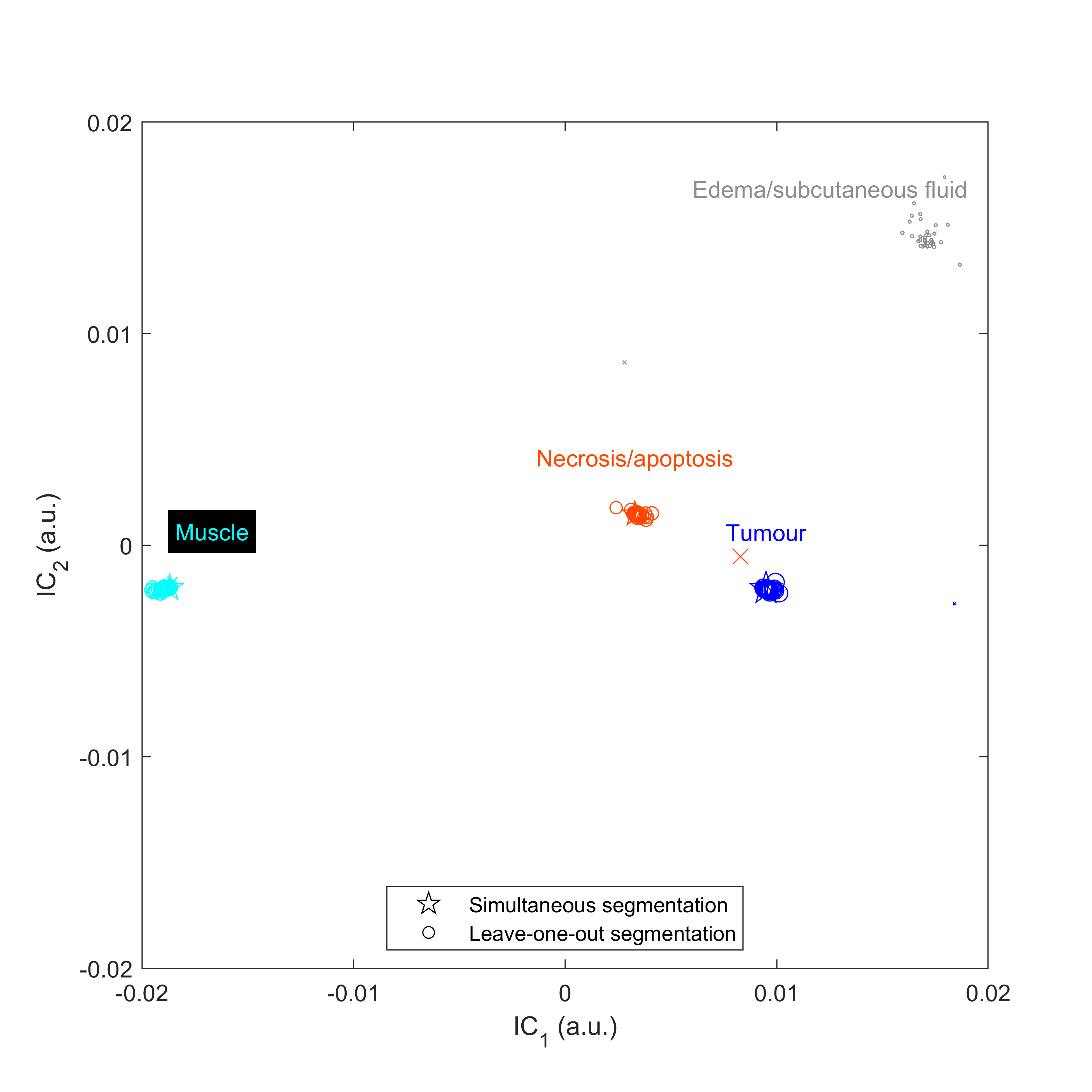
FIGURE 3. Scatter plot of Gaussian mixture model cluster centroids in independent component (IC) space when performing simultaneous (stars) and leave-one-out
segmentation (circles and crosses). The cross represents data from mouse #3 for which leave-one-out
segmentation failed. Symbols are scaled by cluster weight.
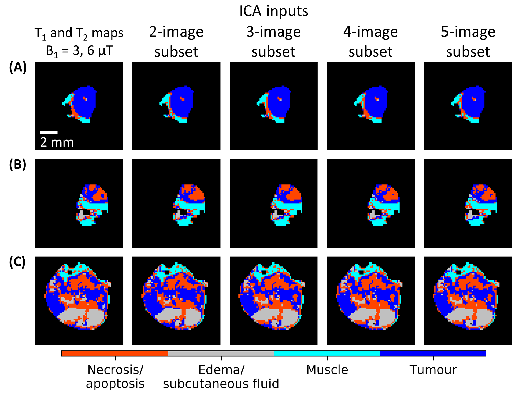
FIGURE 4. Comparison of segmentation using the two- to five-image subsets for the representative cases from Fig. 2. All the masks calculated using image subsets (second to fifth columns) have
an excellent match to the masks calculated using all images (first column). All the masks in this
figure were generated by segmenting the whole dataset (n = 31) simultaneously, i.e., leave-one-out segmentation was not
used here.
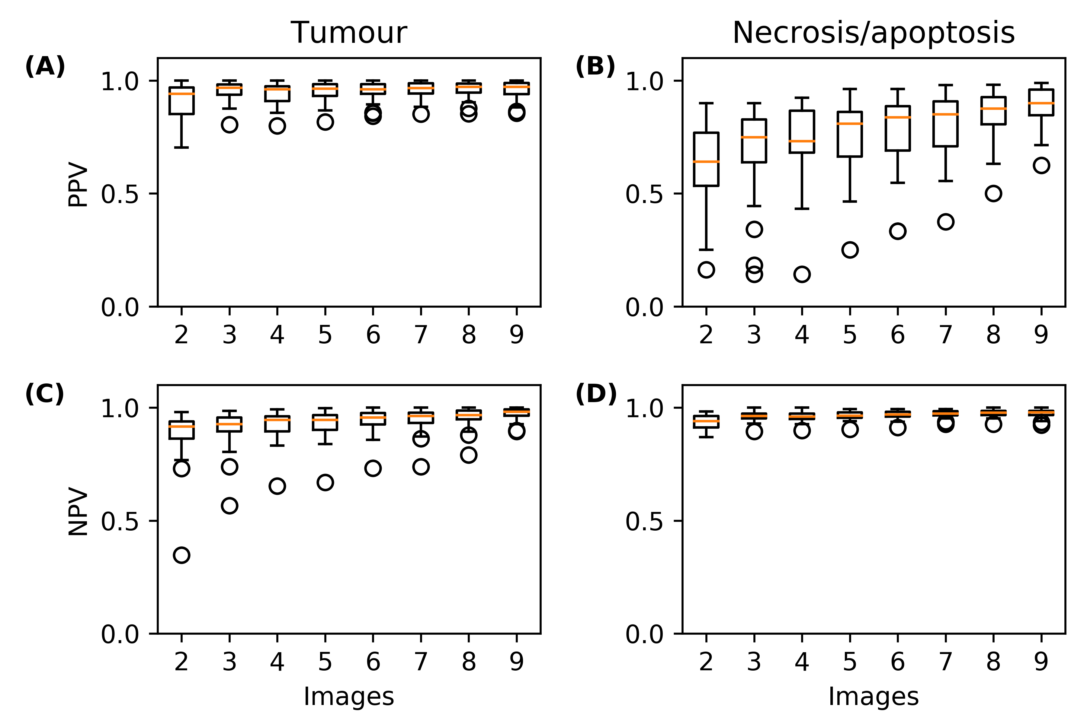
FIGURE 5. Predictive value of automatic segmentation using all the image subsets. Box plots of positive predictive values (PPVs) for (A) tumour-
and (B) necrosis/apoptosis-labelled voxels in the image subsets with respect to
those from segmenting all 24 images simultaneously. (C, D) Similarly, box plots of
negative predictive values (NPVs).