3557
Model uncertainty for MRI segmentation
Andre Maximo1, Chitresh Bhushan2, Dattesh D. Shanbhag3, Radhika Madhavan2, Desmond Teck Beng yeo2, and Thomas Foo2
1GE Healthcare, Rio de Janeiro, Brazil, 2GE Research, Niskayuna, NY, United States, 3GE Healthcare, Bengaluru, India
1GE Healthcare, Rio de Janeiro, Brazil, 2GE Research, Niskayuna, NY, United States, 3GE Healthcare, Bengaluru, India
Synopsis
It is common practice to use dropout layers on U-net segmentation deep-learning models, and it is usually desirable to measure uncertainty of a deployed model while inferencing in clinical scenario. We present a method to convert a pre-trained model to a Bayesian model that can estimate uncertainty by posterior distribution of its trained weights. Our method uses both regular dropouts and converted Monte-Carlo dropouts to estimate uncertainty via cosine similarity of fixed and stochastic predictions. It can identify cases differing from training set by assigning high uncertainty and can be used to ask for human intervention with tough cases.
Introduction
Deep-learning tools are consolidating in various domains, including MR imaging and processing. Two important such tools are: The U-net1, a convolutional neural-network architecture that has become the de facto standard for segmentation tasks; and the dropout layer2, a network layer responsible for randomly zeroing out its input units during the update of training weights to prevent overfitting. Additionally, dropout layers can be used as a Bayesian approximation3 to represent uncertainty in deep-learning models. Normally, dropout layers are used only during training, but they can also be enabled at test time, under the Bayesian approximation3, to produce stochastic predictions instead of fixed predictions. In this scenario, the now Bayesian model is said to contain Monte-Carlo (MC) dropout layers, representing model uncertainty by its posterior distribution of its trained weights.There are many methods to measure model uncertainty using the Bayesian model, depending on the goal and the constraints of the uncertainty measurement. One method is to compute an accuracy metric, such as DICE4, between each stochastic prediction and the ground truth, and measure the spread, i.e. standard deviation, of them5. Another method is to compute the standard deviation per pixel of the stochastic predictions5, producing an uncertainty map that can then be summed and normalized down to a single value. This second method avoids the constrain of having the ground truth. The main limitation of these two methods, and other similar methods in the literature, is the complete disregard of the fixed prediction provided by the non-Bayesian version of the model using regular, i.e. training only, dropout layers. The present work provides a new method to measure model uncertainty using both regular and Monte-Carlo (MC) dropout layers of a U-net model trained to segment brain landmarks in MRI.
Method
The method of this work is to define an uncertainty metric on a model. The model can be an already trained model, there is no need to retrain the model. Although the method has been tested, and results have been drawn, on a U-net model trained to segment MR images of the brain6, the method can be applied to any segmentation model using any neural-network architecture containing dropout layers. The method is applied at test time and it is comprised by two steps (see figure 1 for details). First, the trained model is used in its full, by disabling all dropout layers, to produce a fixed prediction for a given sample. Second, the same trained model is used with partial neurons, by enabling all dropout layers, to produce a set of stochastic predictions for the same given sample. The uncertainty metric for each case is computed via cosine similarity between the fixed prediction and each of the stochastic predictions, cf. equation in the center of figure 1, where u and v are the flatten-out version (one-dimensional) of the probabilities in the fixed and stochastic predictions, respectively. The final uncertainty score is defined as mean of all cosine (dis-)similarities across all stochastic predictions.Results
Four U-net segmentation models6 were used for testing the method: (1) mid-sagittal plane (MSP) segmentation on axial stack of localizer images; (2) plane crossing hippocampus on sagittal stack; (3) MSP segmentation on coronal stack; and (4) pituitary segmentation on sagittal stack. These models were tested using two intrinsically different sets of images: set (A) with 2177 samples, originally used to train and validate all models; set (B) with 25 new samples independent from train/test set that were selected to have characteristics not present in set (A) (e.g. large artifacts due to metal implants, large pathology etc.). For the results, the four models produced one fixed prediction and ten stochastic predictions (n_draws=10 in figure 1) for all samples in all sets. Figures 2 to 4 present the results and are discussed next.Discussions
Figure 2 shows the image input and the stochastic predictions for one subject case from set (B) using first three models. The stochastic predictions are visualized as voxel-wise cumulative sum all predictions before thresholding. Figure 3 shows the distribution of cosine similarity scores on the first three models, in the same sequence of figure 2, for sets (A) and one subject in set (B), interleaved. The low scores for set (A) demonstrate a low uncertainty (i.e. high confidence) for all three models to the same set used while training the models, and the high scores for the subject case in set (B) demonstrate a high uncertainty indicating characteristics that are very different from training datasets, as expected. Figure 4 shows the distribution of cosine similarity scores for the fourth model, comparing sets (A) and (B), further confirming the method in a model that is much more intricate than other and segments a small structure in the brain.Conclusions
Our method can reliably measure uncertainty in predictions from deep-learning models with dropout layers and can assign low confidence values to outputs for cases that differ from training set. This allows runtime identification of cases that may not yield accurate results with the model and can be used to systematically ask for human intervention with tough cases in clinical practice.Acknowledgements
No acknowledgement found.References
- Ronneberger O, Fischer P, Brox T. U-net: Convolutional networks for biomedical image segmentation. In International Conference on Medical image computing and computer-assisted intervention 2015 Oct 5 (pp. 234-241). Springer, Cham.
- Srivastava N, Hinton G, Krizhevsky A, Sutskever I, Salakhutdinov R. Dropout: a simple way to prevent neural networks from overfitting. The journal of machine learning research. 2014 Jan 1;15(1):1929-58.
- Gal Y, Ghahramani Z. Dropout as a Bayesian approximation: Representing model uncertainty in deep learning. In international conference on machine learning 2016 Jun 11 (pp. 1050-1059).
- Milletari F, Navab N, Ahmadi SA. V-net: Fully convolutional neural networks for volumetric medical image segmentation. In 2016 Fourth International Conference on 3D Vision (3DV) 2016 Oct 25 (pp. 565-571). IEEE.
- Do HP, Guo Y, Yoon AJ, Nayak KS. Accuracy, Uncertainty, and Adaptability of Automatic Myocardial ASL Segmentation using Deep CNN. arXiv preprint arXiv:1812.03974. 2018 Dec 10.
- Shanbhag DD et.al. A generalized deep learning framework for multi-landmark intelligent slice placement using standard tri-planar 2D localizers.In Proceedings of ISMRM 2019, Montreal, Canada, p. 670.
Figures
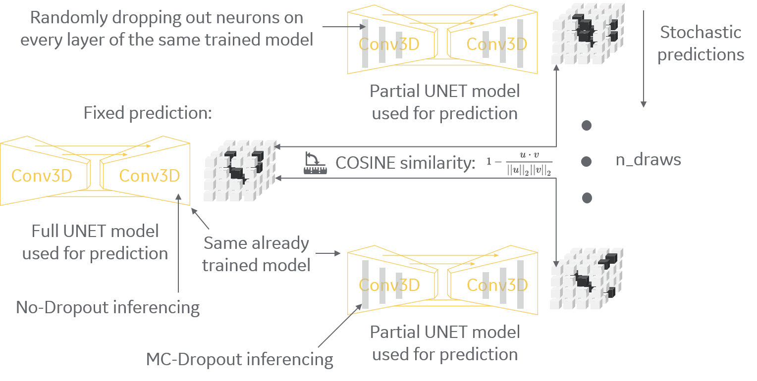
Figure 1: Summary of the
method. While the full U-net model is
used to produce a fixed prediction, partial versions of the same U-net model are
generated by enabling MC dropout layers at test time to produce stochastic
predictions. Model uncertainty is then
defined by the cosine similarity between the fixed prediction and each
stochastic prediction.
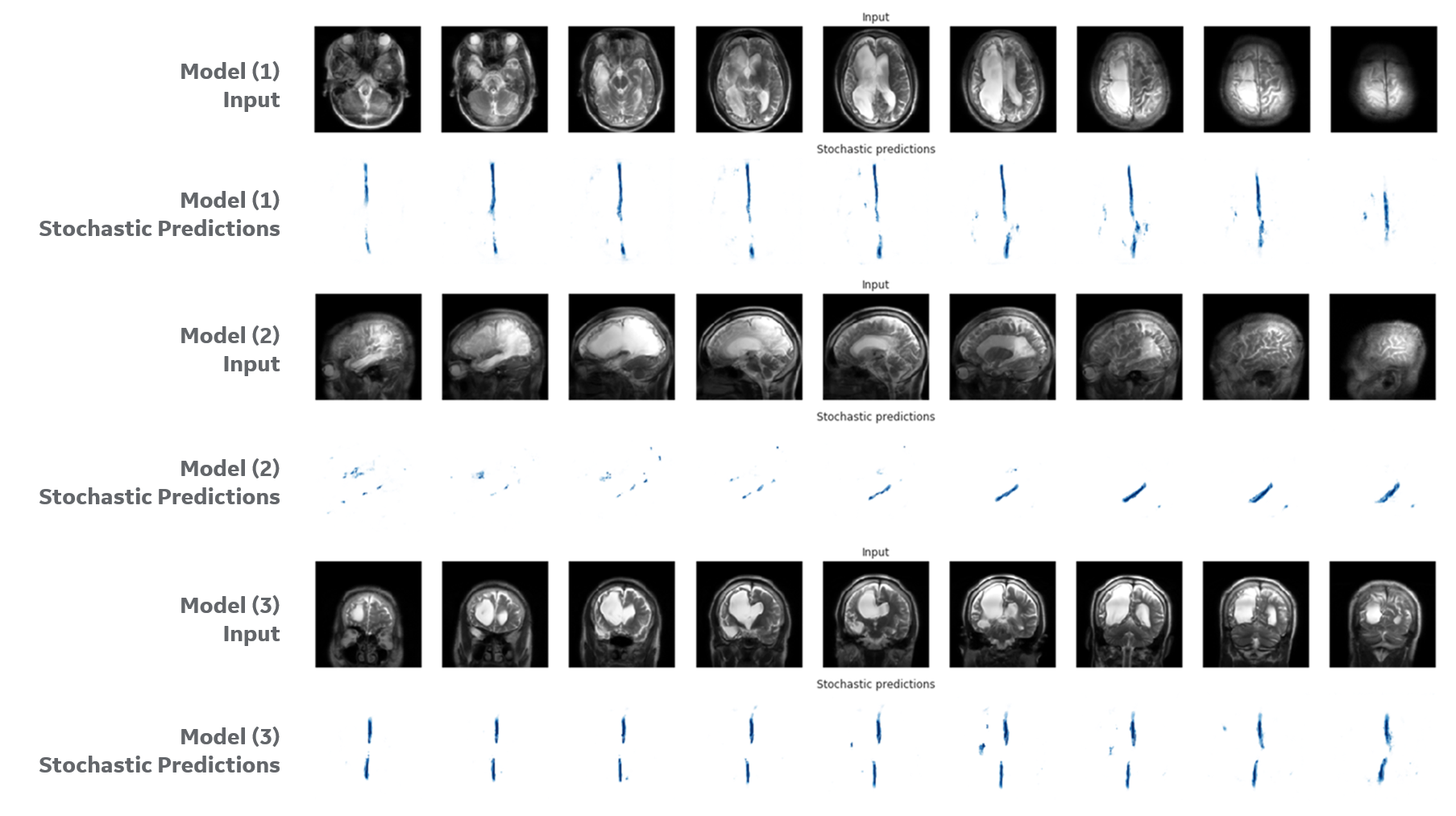
Figure 2: Results on a test subject
case in set (B). Models (1) to (3) have
one row of image input and stochastic predictions output. All stochastic predictions are visualized as voxel-wise
cumulative sum, where white is zero and tones of blue are increasing
positive probabilities (which is desired). Model (1) segments the mid-sagittal plane
landmark in the brain, using an axial stack of images. Model (2) segments a plane crossing the
hippocampus, using a sagittal stack.
Model (3) segments again the mid-sagittal plane on a coronal stack.
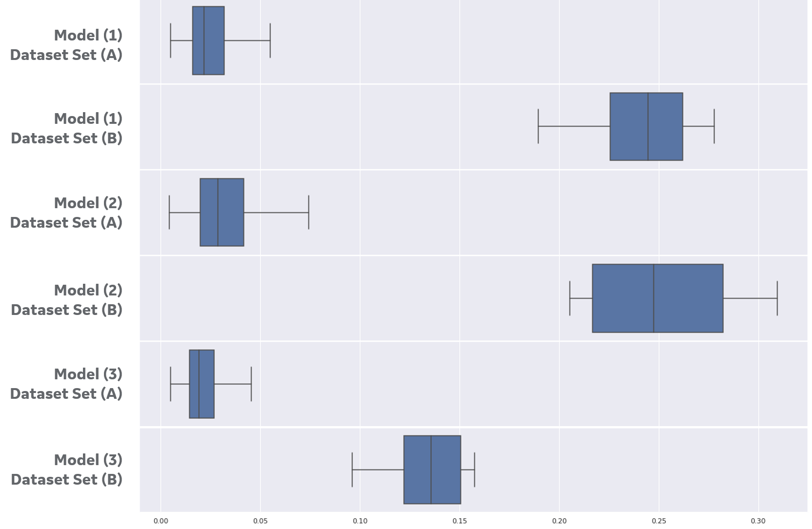
Figure
3: Cosine similarity results on set (A)
compared against one subject case from set (B), illustrated in figure 2, using box-and-whisker
plot. Models (1)-(3) have two rows
each, where the first one shows cosine similarity for train dataset (A) and the
second is the subject from set (B). Note the clear separation between
each pair of distributions. The box
shows the quartiles of the dataset while the whiskers extend to show the rest
of the distribution, except for points that are determined to be "outliers"
using a method that is a function of the inter-quartile range.
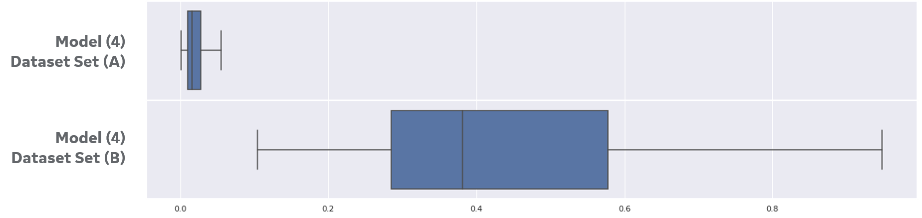
Figure 4:
Cosine similarity results on set (A) compared against the entire set (B) for
model (4) using box-and-whisker plot.
The separation in distributions remain even when segmenting a small structure,
model (4) segments the pituitary in the brain, out of a complex dataset, set
(B) contains 25 subjects with intricate characteristics. The
box shows the quartiles of the dataset while the whiskers extend to show the
rest of the distribution, except for points that are determined to be
“outliers” using a method that is a function of the inter-quartile range.