3548

Visualizing intrinsic magnetic resonance imaging (MRI) dataset variations in image-space through Bayesian deep auto-encoding

Andrew P. Leynes^1,2, Abhejit Rajagopal¹, Valentina Pedoia^1,2, and Peder E.Z. Larson^1,2
¹Radiology and Biomedical Imaging, University of California San Francisco, San Francisco, CA, United States, ²UC Berkeley - UC San Francisco Joint Graduate Program in Bioengineering, Berkeley and San Francisco, CA, United States

Synopsis

We investigated the use of a Bayesian deep auto-encoder to visualize intrinsic variations within a dataset in image-space. The variations were visualized by calculating a voxel-wise standard deviation over the predictions of the Bayesian deep auto-encoder. The low mutual information that was measured between the MRI and the standard deviation maps suggests that new information is contained in the standard deviation maps. This may be useful in the training of deep learning models for anomaly detection.

Introduction

Dataset analysis methods such as t-distributed stochastic neighbor embedding (t-SNE)¹ have allowed for analysis of the relationships of high-dimensional data. However, it is unclear how to visualize variations of the dataset on the image itself. Unsupervised analysis of variation can have great impact in adding interpretability to machine learning models and help the community in gaining trust in image translation and restoration tasks solved with encoder-decoder architectures. In addition, unsupervised analysis of variation allows the possibility to study the overall variation in datasets that is often confounded with the task of interest. In this work, we demonstrate that training a Bayesian deep auto-encoder on a MRI dataset allows for visualization of intrinsic image variations. The voxel-wise standard deviation map highlights and localizes regions of high variation relative to the entire dataset in image-space.

Methodology

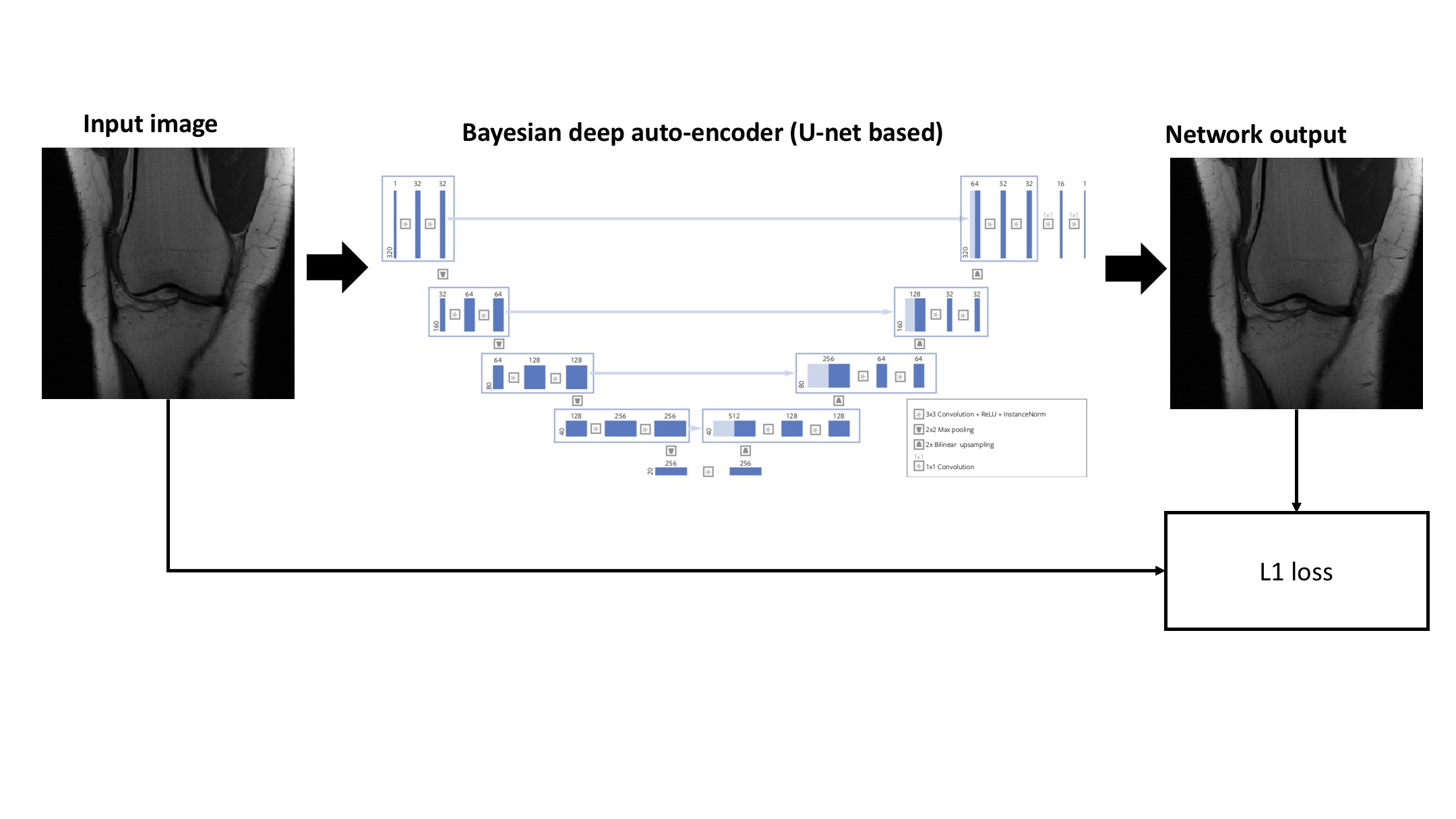
Dataset: The fastMRI dataset² consists of 34,742 2D coronal image slices of clinical patients who had knee MRI scans at the New York University (NYU) School of Medicine. There were approximately 50% proton-density knee MRI and approximately 50% fat-suppressed proton-density knee MRI acquired on different scanner configurations (Skyra 3T, Prisma 3T, Biograph mMR 3T, and Aera 1.5T).
Network and training: The Bayesian deep auto-encoder (BDA) architecture was based on U-net³ with the addition of Dropout (p=0.1) layers⁴. The network inputs were magnitude images and the network was trained to reconstruct the same magnitude images with an L1 loss. An Adam optimizer was used and the network was trained for 30 epochs. A flowchart of the training procedure is shown in Figure 1. The network was trained on fully sampled sum-of-squares images from the fastMRI dataset under the “singlecoil” challenge².
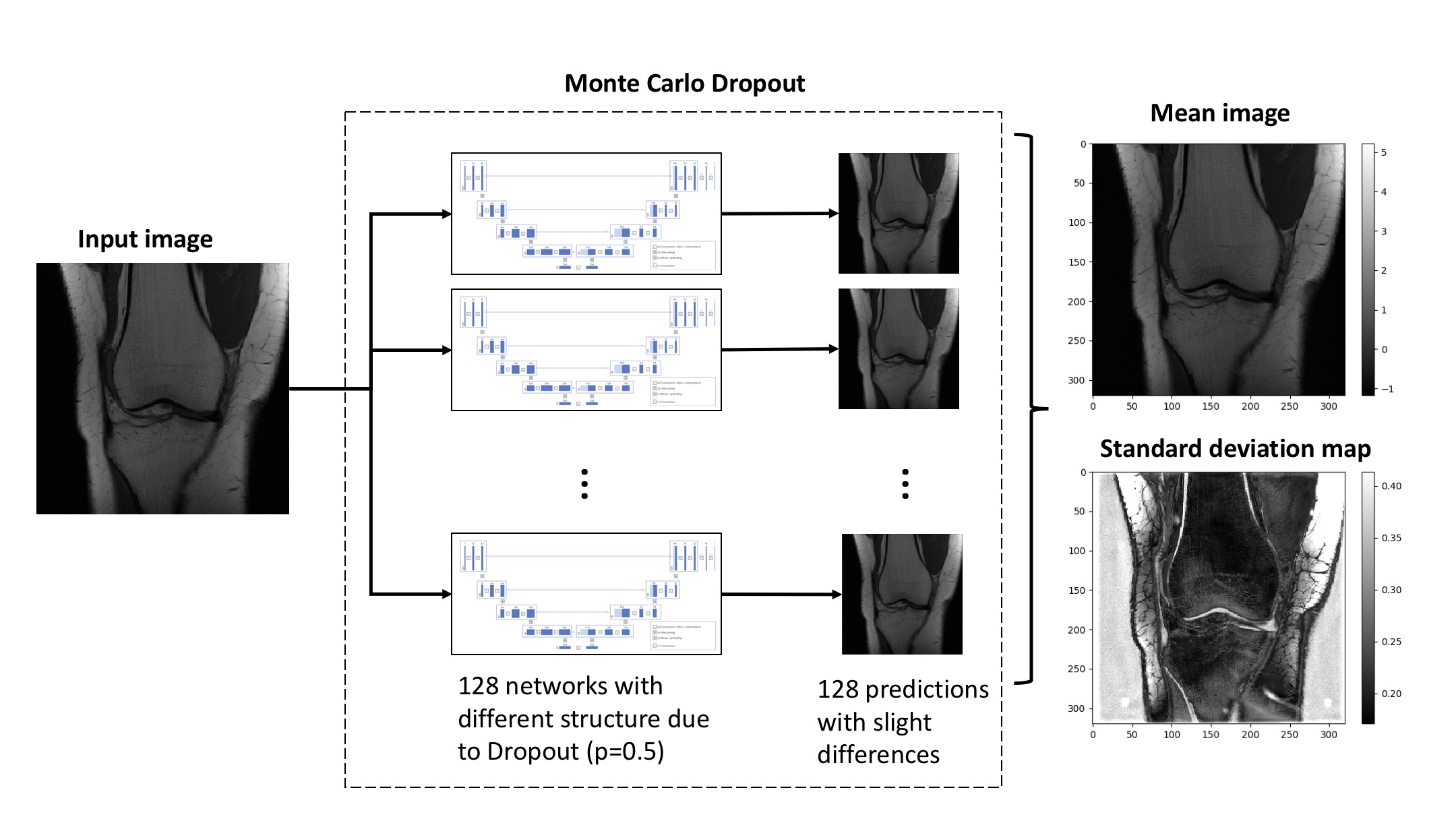
Inference and testing: Using the validation dataset of the “singlecoil” fastMRI dataset, several images were processed using the BDA. Monte Carlo Dropout⁵ (MC Dropout) was used to convert the U-net auto-encoder to a Bayesian deep auto-encoder. Inference was performed with Monte Carlo Dropout (p=0.5) with 128 forward passes. The process for Monte Carlo Dropout is shown in Figure 2. The standard deviation map was derived by computing a voxel-wise standard deviation. Self-information and mutual information was calculated using a 2D-histogram method with 32 bins.

Results

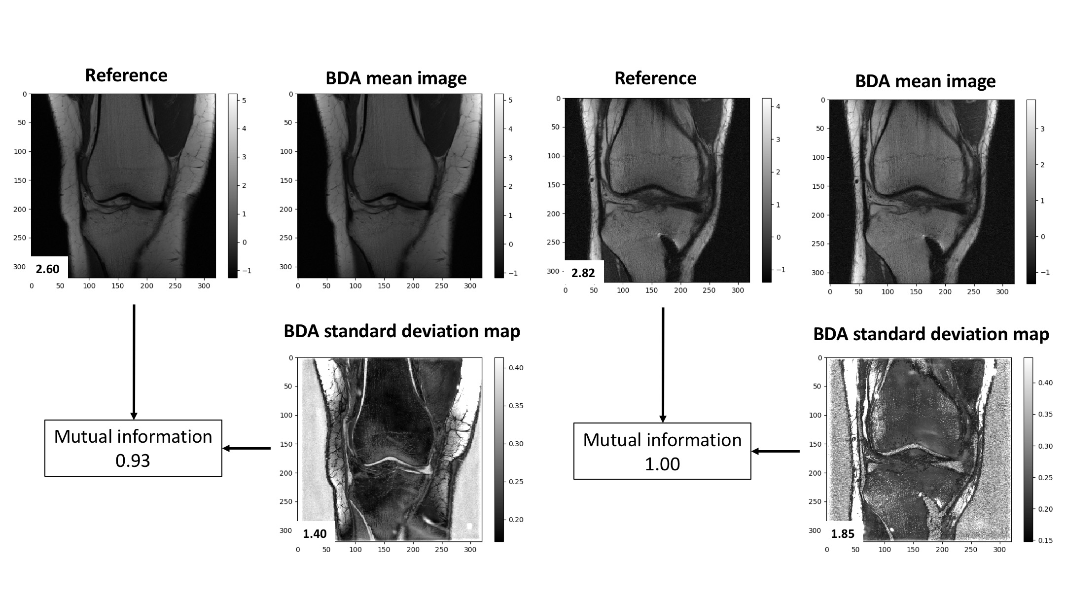
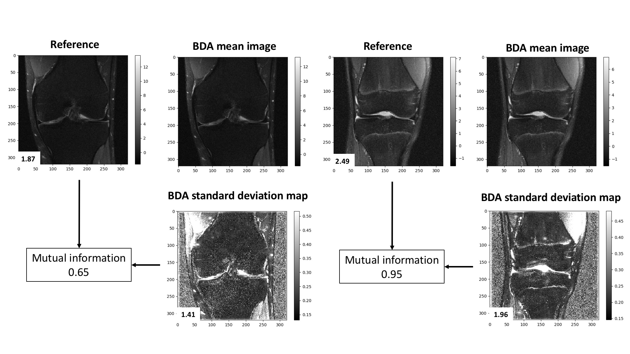
Figure 3 shows images of a coronal proton-density knee MRI alongside the standard deviation maps produced by the Monte Carlo Dropout. The standard deviation map highlights regions of low spatial frequency signal intensity variations such as those due to coil sensitivity profiles and bone marrow density. It also highlights some low signal regions around the cortical bone, the deep layers of cartilage, and the meniscus.
Figure 4 shows images of a coronal proton-density fat suppressed knee MRI alongside the standard deviation maps produced by the Monte Carlo Dropout. In addition to the features highlighted in Figure 3, the standard deviation map in these cases additionally highlights abnormalities of fluid within the joint and the prominent growth plates. In all cases, since the mutual information is less than the self-information of the original image and the BDA standard deviation map, this suggests that the standard deviation maps have additional unique information.

Conclusions

We proposed a method for analyzing intrinsic MRI dataset variations in image-space through a Bayesian deep auto-encoder. The standard deviation maps highlights and localizes image regions that differ from some learned population mean, such as MRI acquisition variations (e.g. coil sensitivity profile) or biological variations (e.g. abnormalities of fluid within the joint). This map may serve as an additional contrast mechanism and may provide additional information for the training of deep learning based anomaly or artifact detection models.

Acknowledgements

This project was supported in part by the UCSF Graduate Research Mentorship Fellowship award. The Titan X Pascal used was donated by the NVIDIA Corporation.

References

1. L. van der Maaten and G. Hinton, Visualizing Data using t-SNE, Journal of Machine Learning Research 9(Nov), 2579–2605 (2008).

2. J. Zbontar, F. Knoll, A. Sriram, et al., fastMRI: An Open Dataset and Benchmarks for Accelerated MRI, arXiv:1811.08839 [physics, stat] (2018).

3. O. Ronneberger, P. Fischer, and T. Brox, U-Net: Convolutional Networks for Biomedical Image Segmentation, in Medical Image Computing and Computer-Assisted Intervention – MICCAI 2015(Springer, Cham, 2015), pp. 234–241.

4. N. Srivastava, G. Hinton, A. Krizhevsky, I. Sutskever, and R. Salakhutdinov, Dropout: A Simple Way to Prevent Neural Networks from Overfitting, J. Mach. Learn. Res. 15(1), 1929–1958 (2014).

5. Y. Gal and Z. Ghahramani, Dropout as a Bayesian Approximation: Representing Model Uncertainty in Deep Learning, arXiv:1506.02142 [cs, stat] (2015).

Figures

Figure 1. Bayesian deep auto-encoder architecture and training. The network was based on the U-net implementation of Zbontar et al². The network was trained to reconstruct the same input image with an L1-loss.

Figure 2. Prediction with the Bayesian deep auto-encoder was performed using Monte Carlo Dropout. The mean image is the voxel-wise mean of the different predictions and the standard deviation map is the voxel-wise standard deviation of the different predictions.

Figure 3. Predictions and measurement of mutual information on coronal proton-density knee MRI. The self-information of the reference image and standard deviation maps are shown in the bottom-left corner of each image. The standard deviation map highlights regions of low spatial frequency signal intensity variations such as those due to coil sensitivity profiles and bone marrow density. It also highlights some low signal regions around the cortical bone, the deep layers of cartilage, and the meniscus.

Figure 4. Predictions and measurement of mutual information on coronal fat suppressed proton-density knee MRI. The self-information of the reference image and standard deviation maps are shown in the bottom-left corner of each image. The standard deviation maps highlights regions of low spatial frequency signal intensity variations such as those due to coil sensitivity profiles. It also highlights abnormalities of fluid within the joint and the prominent growth plates.

Proc. Intl. Soc. Mag. Reson. Med. 28 (2020)

3548