3547
Deep Learning-based Perfusion Parameter Mapping (DL-PPM) with Simulated Microvascular Network Data
Liangdong Zhou1, Jinwei Zhang1,2, Qihao Zhang1,2, Pascal Spincemaille1, Thanh D Nguyen1, Yi Wang1,2, and Liangdong Zhou3
1Weill Medical School of Cornell University, New York, NY, United States, 2Cornell University, Ithaca, NY, United States, 3Radiology, Weill Medical School of Cornell University, New York, NY, United States
1Weill Medical School of Cornell University, New York, NY, United States, 2Cornell University, Ithaca, NY, United States, 3Radiology, Weill Medical School of Cornell University, New York, NY, United States
Synopsis
Perfusion parameters, including blood flow (BF), apparent blood velocity (V), blood volume (BV) and arterial transit time (ATT) are useful for the disgnosis of many dieases. Typically, perfusion quantification methods utilize the tracer concentration (ASL, DEC, DSC, etc.) as input and blood flow map as output. We proposed a deep learning-based perfusion parameters mapping (DL-PPM), which uses 4D time-revolved tracer concentration as input and perfusion parameters (BF, V, BV, ATT) as output. We tested the propose method using simulated data and in vivo data in kidney.
Introduction
Blood perfusion quantification is of essential importance for the diagnosis of many diseases, including stroke, heart attack, cancer, Alzheimer’s disease and other diseases that affect blood flow. Perfusion parameters, including blood flow (BF), apparent blood velocity (V), blood volume (BV) and arterial transit time (ATT) are useful for the diagnosis of many diseases1-5. Typically, perfusion quantification methods utilize the tracer concentration (ASL, DEC, DSC, etc.) as input and blood flow map as output6. Mapping all the perfusion parameters mentioned from one dataset using the conventional perfusion quantification method could be challenging. We proposed a deep learning-based perfusion parameter mapping (PPM), which uses a dataset of simulated 4D time series of tracer concentration as input and produces perfusion parameters (BF, V, BV, ATT)7,8. To validate DL-PPM method, we simulated a microvascular network in the kidney and the corresponding blood velocity using the Navier-Stokes equation and tracer concentration based on mass transport equation9. The ground truth of the perfusion parameters was calculated from the simulation settings and served as a training label. A recurrent neural network (RNN) was used to capture the data relation between time frames.Methods and material
$$${\bf 1.\,Numerical\,simulation\,for\,training\,data}$$$The blood velocity in the microvascular network follows the static state Navier-Stokes equation10
$$\rho_b({\bf\,u}\cdot\nabla){\bf\,u}\,=\,\nabla\,p+\mu\nabla\cdot\nabla{\bf\,u},\,\quad{\bf\,r}\in\Omega_v,\qquad\,(1)$$ $$\rho_b\nabla\cdot{\bf\,u}=0,\,\quad{\bf\,r}\in\Omega_v,\,\qquad(2)$$ in which $$$\rho_b$$$ is the blood density, $$$p$$$ the blood pressure, $$$\mu$$$ the blood viscosity, and $$$\Omega_v$$$ the intravascular space. The blood pulsation was ignored for simplicity.
Assume that the blood tracer has the same velocity as the blood. The tracer concentration $$$c({\bf r},t))$$$ in the blood vascular space is governed by the mass transport equation11
$$\partial_tc({\bf\,r},t)=-\nabla\cdot(c({\bf\,r},t){\bf\,u}({\bf\,r}))+\nabla\cdot(D({\bf\,r})\nabla\,c({\bf r},t))-\gamma\,c({\bf\,r},t),\quad {\bf\,r}\in\Omega_v,\,(3)$$ where $$$D$$$ is the diffusion coefficient, $$$\gamma$$$ is the tracer signal decay rate.
$$${\bf 2.\,Recurrent\,neural\,network}$$$
As the constructed ground truth of the perfusion parameters $$$G=(BF, V, BV, ATT)$$$ and the simulated tracer concentration data $$$C({\bf r},t)$$$ were obtained, the recurrent neural network (RNN) was feed with $$$(G, C_{t_i}), i = 1, \ldots,N$$$ data pairs for training and validation, where $$$i$$$ is the time indicator and $$$N$$$ is the total number of time frames12. $$S_i=f(S_{i-1}W_{rec }+C_{t_i}W_c),\qquad(4)$$ where $$$S_i$$$ is the state at the time $$$t_i$$$, $$$C_{t_i}$$$ the exogenous input at time $$$t_i$$$, $$$W_{rec}$$$ and $$$W_c$$$ are weight parameters like that in feedforward net. The fitting term to optimize during the training is defined as $$\min_{W_{rec}, W_c}\|Y_N-G\|_2.$$ Stochastic gradient descent on image patches was used during the training.
$$${\bf 3.\,In\,vivo\,experiments}$$$
Renal arterial spin labeling (ASL) data was acquired with multiple post-labeling delays (PLD) for seven healthy volunteers. The data acquisition parameters are: 3D FSE PCASL, GE MR750 3T scanner, 32 channel body coil, 2.5x2.5x4 mm3 voxel size, 128x128x36 matrix size, 10.4840ms TE, 111o flip angle, three signal averages, ~4.5 min scan time, PLD = 1025ms, 1525ms, 2025ms, 2525ms, background suppression, synchronized breathing. At the same image acquisition session, non-contrast 3D MR angiogram (MRA) IFIR data were acquired for each subject. Acquisition parameters for the MRA include: 0.625x0.625x2 mm3 voxel size, 512x512x128 matrix size, 4.0240ms TR, 2.0120ms TE, 50o flip angle, with breath gating13.
The numerical microvascular network for each volunteer was constructed based on the hemodynamic principles with the anatomical information from ASL, M0 and MRA images. The blood volume (BV) is computed from the microvascular network structure. These microvascular networks serve as the domain for equations (1)-(3). Therefore, the velocity (V), tracer concentration (C) can be calculated by solving (1)-(3). ATT is obtained from the dynamics of tracer transportation. The blood flow (BF) is computed from the velocity and the microvascular network cross-sectional area. All of these parameters (BF, V, BV, ATT) were then voxelized to the image voxel scale and set as the ground truth (label image for training).
Results
Figure 1. shows the RNN architecture used for the training. There are four input layers corresponding to the four PLDs of ASL data used.Figure 2. presents the numerical simulation solutions in the microvascular network. The ground truth of RBV is generated from the simulated microvasculature, blood velocity (V) and flow (BF) are generated from the voxelization of (b) and (c), ATT was captured from the time curve of tracer concentration. These perfusion parameters ground truth and voxelized tracer concentration data together serve as the training data.
Figure 3. displays the reconstruction results from the proposed DL-PPM and the comparison of the results between DL-PPM, Kety’s method3,14 and the ground truth.
Figure 4. shows the quantitative estimation of the reconstruction error for DL-PPM and Kety’s method in Figure 3.
Figure 5. shows the application of trained DL-PPM to in vivo health volunteer data. The results were compared with the conventional Kety’s method.
Discussion and conclusion
The preliminary results from the numerically simulated data and the in vivo data show that DL-PPM is able to generate four perfusion parameters (BF, V, BV, ATT) from the multiple PLDs ASL data with acceptable accuracy. The quantitative analysis of the blood velocity and flow implies that DL-PPM outperforms Kety’s method. DL-PPM quantifies the perfusion parameters without using assumptions that are generally required in Kety’s method15. And DL-PPM does not need the AIF which might introduce bias or errors in the conventional perfusion quantification methods.Acknowledgements
No acknowledgement found.References
- Zhou L, Spincemaille P, Zhang Q, Nguyen T, Doyeux V, Lorthois S, Wang Y. Vector Field Perfusion Imaging: A Validation Study by Using Multiphysics Model. Proc. Intl. Soc. Mag. Reson. Med. 26 (2018), P.1870.
- Zhang Q, Spincemaille P, Zhou L, Morgan J, Jafari R, Hubertus S, Fakultat M, Eskreis-Winkler S, Nguyen T, Zhang S, Kovanlikaya I, Tsiouris A, Margolis D, Sutton E, Gupta A, Morris E, Prince M, Wang Y. Quantitative Transport Mapping (QTM): Inverse Solution to a Voxelized Equation of Mass Flux in a Porous Tissue Model. Magn Reson in Med, Under review 2019.
- Alsop DC, Detre JA, Golay X, Gunther M, Hendrikse J, Hernandez-Garcia L, Lu H, MacIntosh BJ, Parkes LM, Smits M, van Osch MJ, Wang DJ, Wong EC, Zaharchuk G. Recommended implementation of arterial spin-labeled perfusion MRI for clinical applications: A consensus of the ISMRM perfusion study group and the European consortium for ASL in dementia. Magnetic resonance in medicine 2015;73(1):102-116.
- Akhbardeh A, Sagreiya H, El Kaffas A, Willmann JK, Rubin DL. A multi-model framework to estimate perfusion parameters using contrast-enhanced ultrasound imaging. Medical Physics 2019;46(2):590-600.
- McKinley R, Hung F, Wiest R, Liebeskind DS, Scalzo F. A Machine Learning Approach to Perfusion Imaging With Dynamic Susceptibility Contrast MR. Front Neurol 2018;9.
- Wang Z. Support vector machine learning-based cerebral blood flow quantification for arterial spin labeling MRI. Hum Brain Mapp 2014;35(7):2869-2875.
- Calamante F, Gadian DG, Connelly A. Quantification of perfusion using bolus tracking magnetic resonance imaging in stroke - Assumptions, limitations, and potential implications for clinical use. Stroke 2002;33(4):1146-1151.
- Buxton RB, Frank LR, Wong EC, Siewert B, Warach S, Edelman RR. A general kinetic model for quantitative perfusion imaging with arterial spin labeling. Magnetic resonance in medicine 1998;40(3):383-396.
- Zhou L, Zhang Q, Spincemaille P, Nguyen T, Wang Y. Quantitative Transport Mapping (QTM) of the Kidney using a Microvascular Network Approximation. Proc. Intl. Soc. Mag. Reson. Med. 27 (2019), P.703.
- Secomb TW. Hemodynamics. Compr Physiol 2016;6(2):975-1003.
- Chen JS, T. CJ, W. LC, P. LC, W LC. Analytical solutions to two-dimensional advection–dispersion equation in cylindrical coordinates in finite domain subject to first- and third-type inlet boundary conditions. Journal of Hydrology 2011;405:10.
- Qin C, Schlemper J, Caballero J, Price AN, Hajnal JV, Rueckert D. Convolutional Recurrent Neural Networks for Dynamic MR Image Reconstruction. IEEE transactions on medical imaging 2019;38(1):280-290.
- Rajendran R, Lew SK, Yong CX, Tan J, Wang DJJ, Chuang KH. Quantitative mouse renal perfusion using arterial spin labeling. NMR in biomedicine 2013;26(10):1225-1232.
- Robson PM, Madhuranthakam AJ, Smith MP, Sun MR, Dai W, Rofsky NM, Pedrosa I, Alsop DC. Volumetric Arterial Spin-labeled Perfusion Imaging of the Kidneys with a Three-dimensional Fast Spin Echo Acquisition. Acad Radiol 2016;23(2):144-154.
- Calamante F. Arterial input function in perfusion MRI: a comprehensive review. Prog Nucl Magn Reson Spectrosc 2013;74:1-32.
Figures
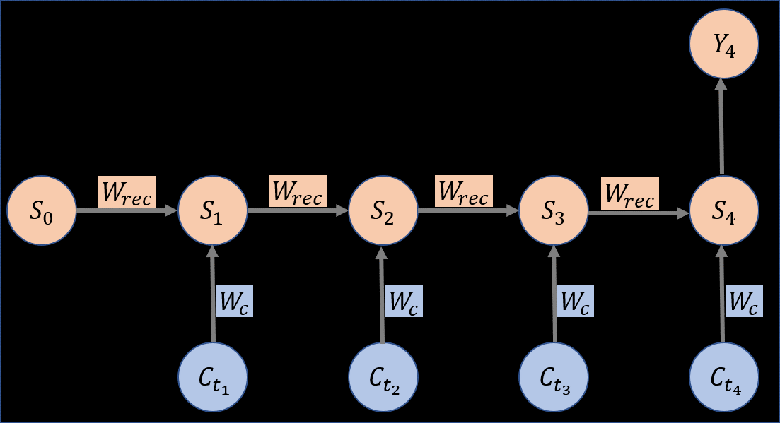
Figure 1: The recurrent neural network used in this work. Four input layers with $$$C_{t_i}, i = 1,2,3,4$$$ as inputs since ASL data with four post labeling delay was used. $$$W_{rec}$$$ and $$$W_c$$$ are trainable parameters and $$$Y_4$$$ is the output of the network, which in this work is the perfusion parameters (BF,
V, BV, ATT) .
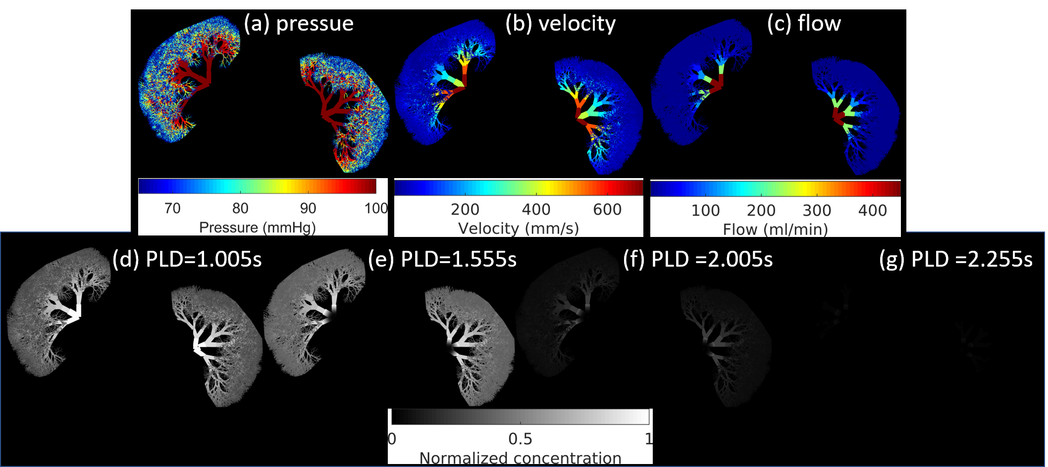
Figure
2:
The numerical simulation solutions in the microvascular
network. (a)-(c) are the blood pressure, blood velocity and blood flow in the
vascular network by solving the Navier-Stokes equation. (d)-(g) are the tracer
concentration at four PLDs simulated from the transport equation with the
velocity in (b).
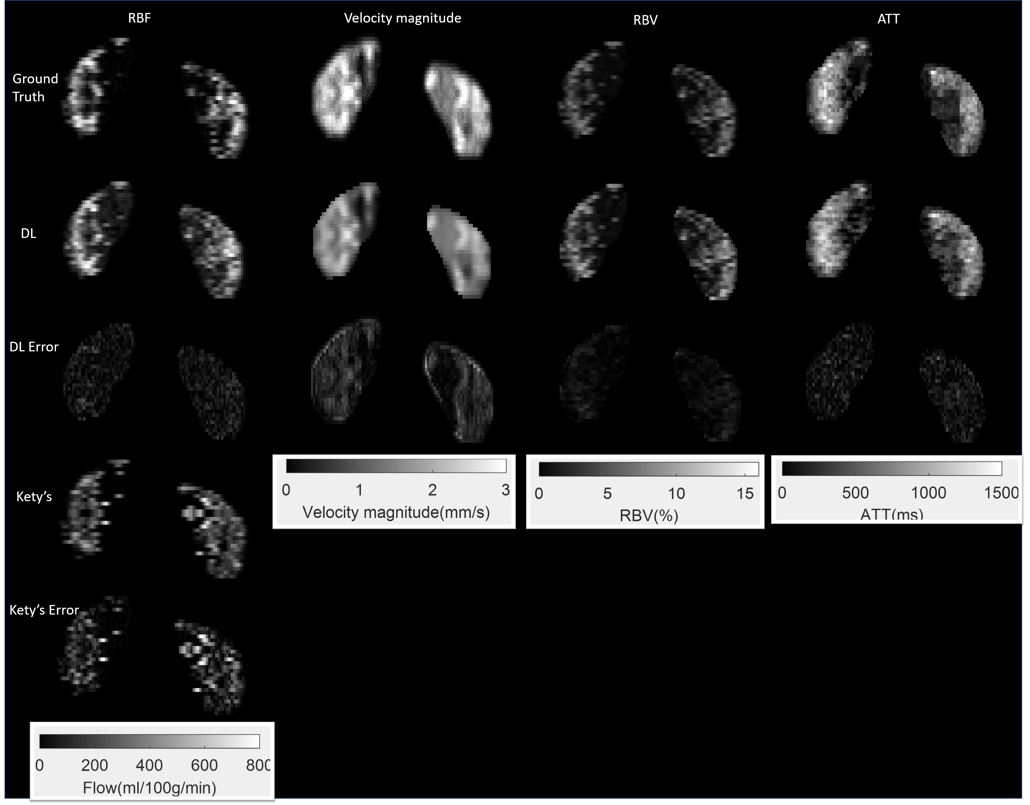
Figure
3: Perfusion parameters reconstructed using the DL-PPM,
and the results comparison with ground truth and Kety’s method. Column 1 to
column 4 are renal blood flow (RBF), blood velocity magnitude, renal blood
volume (RBV), and arterial transit time (ATT), respectively. Row 1 to row 5 are
the ground truth, deep learning results, deep learning error maps, Kety’s
method results, and Kety’s results error maps, respectively.
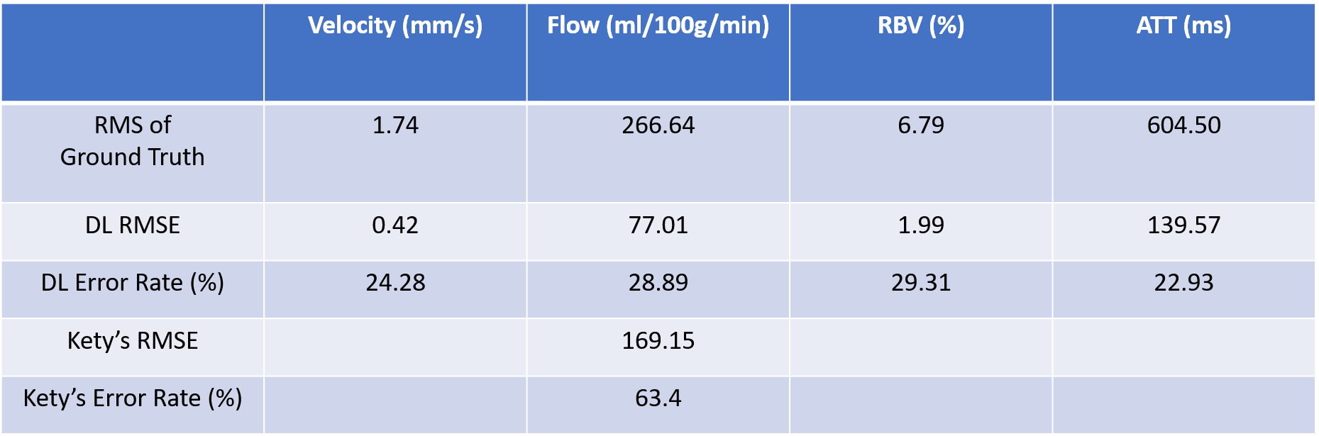
Figure
4:
Perfusion parameters error of the deep learning results. There are consistent
errors for all the four parameters from DL-PPM. It also shows that flow errors
from Kety’s method are more than tow fold of that from DL-PPM.
Figure
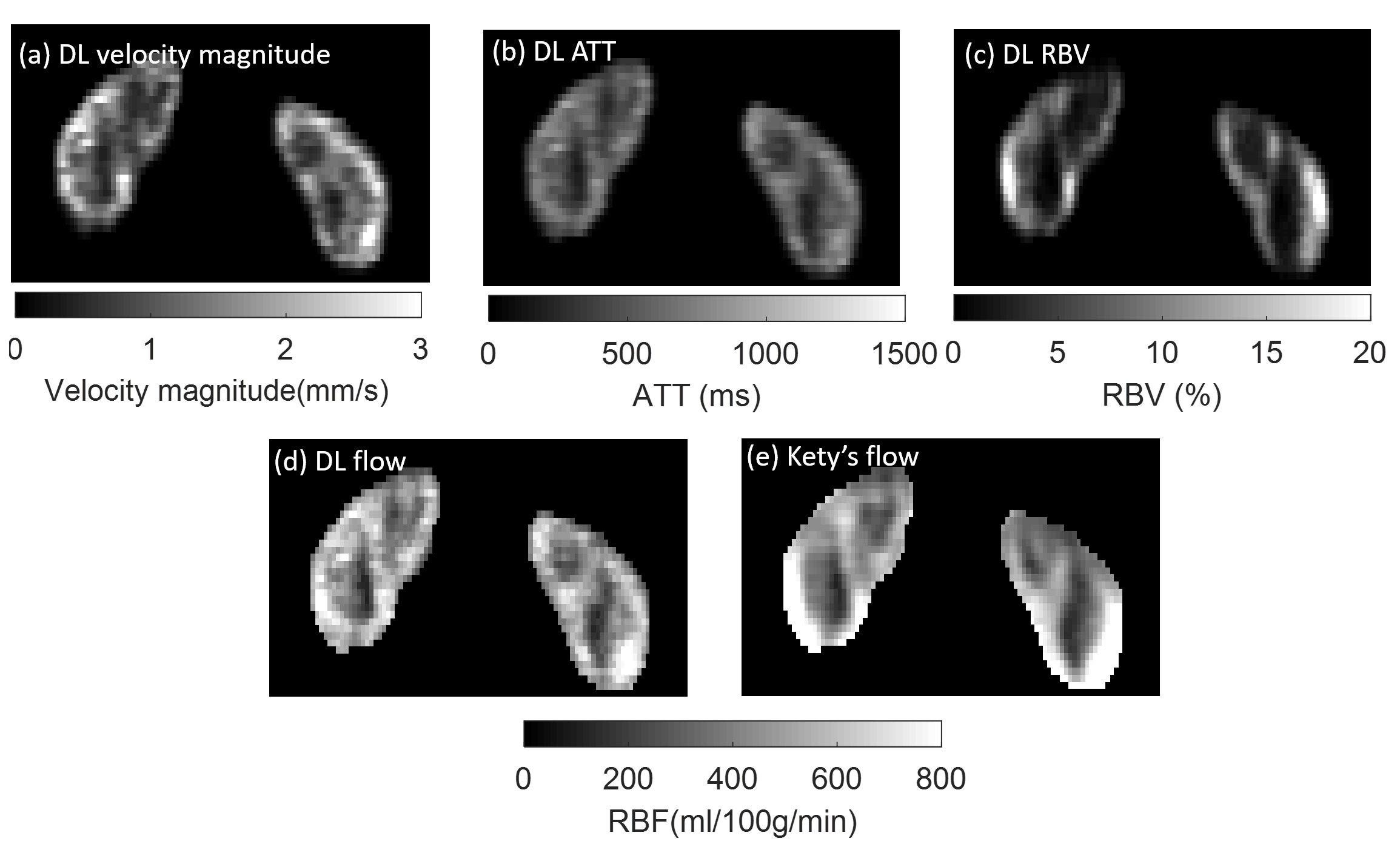
5: DL-PPM results for in vivo ASL data. (a)-(d)
are the results of DL-PPM. (e) is the flow map from Kety’s method. It shows
that Kety’s flow map is less homogeneous than the flow from DL-PPM in the cortex region, which could
potentially result from the artifacts in the M0 image.