Introduction

Deep learning-based methods, which have shown impressive outcomes in various fields, have been studied in association with synthetic MR image. Recently, MR image synthesis methods using multi contrast input images show improved performances. However, multi-contrast images obtained from the same subject may have slight positional differences (misregistration) because they are scanned sequentially rather than by a single sequence. To minimize these differences, subjects are requested not to move, but various inevitable movements due to breathing and blood vessel phase changes, etc., may cause small errors in alignment that cannot be easily compensated with even the most advanced registration algorithms¹. However, this slight misregistration can cause blurring or loss of detail in deep-learning processes². Therefore, we proposed a special deep learning loss function for processing multiple image.

Methods

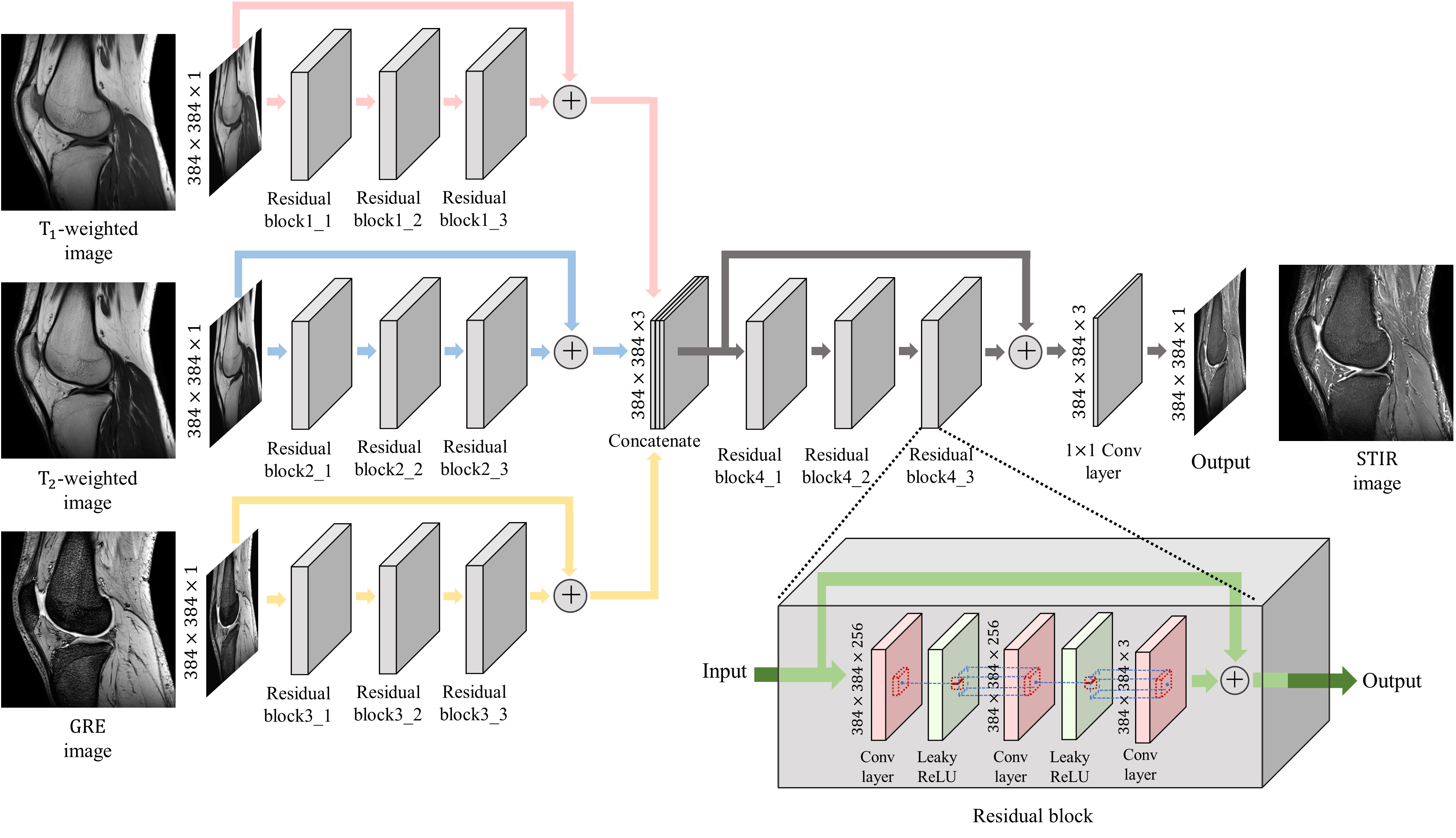
We aimed to infer STIR images from T1-w, T2-w, and GRE images through a deep neural network, which is a suitable architecture for estimating highly non-linear relationships among signals. Figure. 1 shows the overall architecture of our proposed CC-DNN model. The activation function used in our CC-DNN is the leaky-rectified linear unit function. Each convolutional layer except the final one is followed by a batch normalization layer. And adam³ optimizer is used to train our model with a learning rate as 0.0001.
The CC-DNN model is optimized by our proposed loss function, which consists of three loss components. The first one is the mean squared error (MSE) function, which is expressed by the following equation:
(1) $$ c_{1}(I_{STIR},\widehat{I_{STIR}}) = \frac{1}{w\times h} \sum_{i=1}^{w}\sum_{j=1}^{h}(I_{STIR}[i,j]-\widehat{I_{STIR}}[i,j])^{2} $$
This loss component optimizes the CC-DNN model by reducing the intensity differences of all pixels of $$$I_{STIR} $$$ and $$$\widehat{I_{STIR}}$$$. The second loss component considers the surroundings when it calculates the intensity difference of each pixel. It calculates intensity differences between the output pixel and its k×k surrounding pixels of the label image and keeps only minimum differences. The second loss component is expressed as the following equation:
(2) $$ c_{2}(I_{STIR},\widehat{I_{STIR}}) = \frac{1}{w\times h} \sum_{i=\left \lfloor \frac{k}{2} \right \rfloor+1}^{w-\left \lfloor \frac{k}{2} \right \rfloor}\sum_{j=\left \lfloor \frac{k}{2} \right \rfloor+1}^{h-\left \lfloor \frac{k}{2} \right \rfloor} min(M_{i,j}-\widehat{I_{STIR}}[i,j]\times J)^{2} ,$$
$$ M_{i,j} = \begin{bmatrix}I_{STIR}\left [ i -\left \lfloor \frac{k}{2} \right \rfloor,j-\left \lfloor \frac{k}{2} \right \rfloor \right ] & \cdots & I_{STIR}\left [ i -\left \lfloor \frac{k}{2} \right \rfloor,j+ \left \lfloor \frac{k}{2} \right \rfloor \right ]\\ \vdots & \ddots & \vdots \\ I_{STIR}\left [ i +\left \lfloor \frac{k}{2} \right \rfloor,j-\left \lfloor \frac{k}{2} \right \rfloor \right ] & \cdots & I_{STIR}\left [ i +\left \lfloor \frac{k}{2} \right \rfloor,j+\left \lfloor \frac{k}{2} \right \rfloor \right ]\end{bmatrix} $$
where $$$J\in R^{k\times k}$$$ is an all-ones matrix. The third loss component compensates for this by minimizing the differences in local average and the local variation between the output and the label images. This allows the generated $$$\widehat{I_{STIR}}$$$ to learn the complex structural diversity of $$$I_{STIR}$$$. The third loss component is expressed as the following equation:
(3) $$c_{3}\left ( I_{STIR},\widehat{I_{STIR}} \right ) = \frac{1}{w\times h}\sum_{i=3}^{w-2}\sum_{j=3}^{h-2}(var(M_{i,j})-var(N_{i,j}))^2,$$
$$N_{i,j} = \begin{bmatrix}\widehat{I_{STIR}}\left [ i - 2, j-2 \right ] & \cdots & \widehat{I_{STIR}}\left [ i - 2, j+2 \right ]\\ \vdots & \ddots & \vdots \\ \widehat{I_{STIR}}\left [ i + 2, j-2 \right ] & \cdots & \widehat{I_{STIR}}\left [ i + 2, j+2 \right ]\end{bmatrix}$$
The proposed loss function is defined as a weighted summation of three loss components, which can be represented as follows: $$$Loss = c_{1}+0.3\times c_{2} +0.3\times c_{3}$$$

Result and Discussion

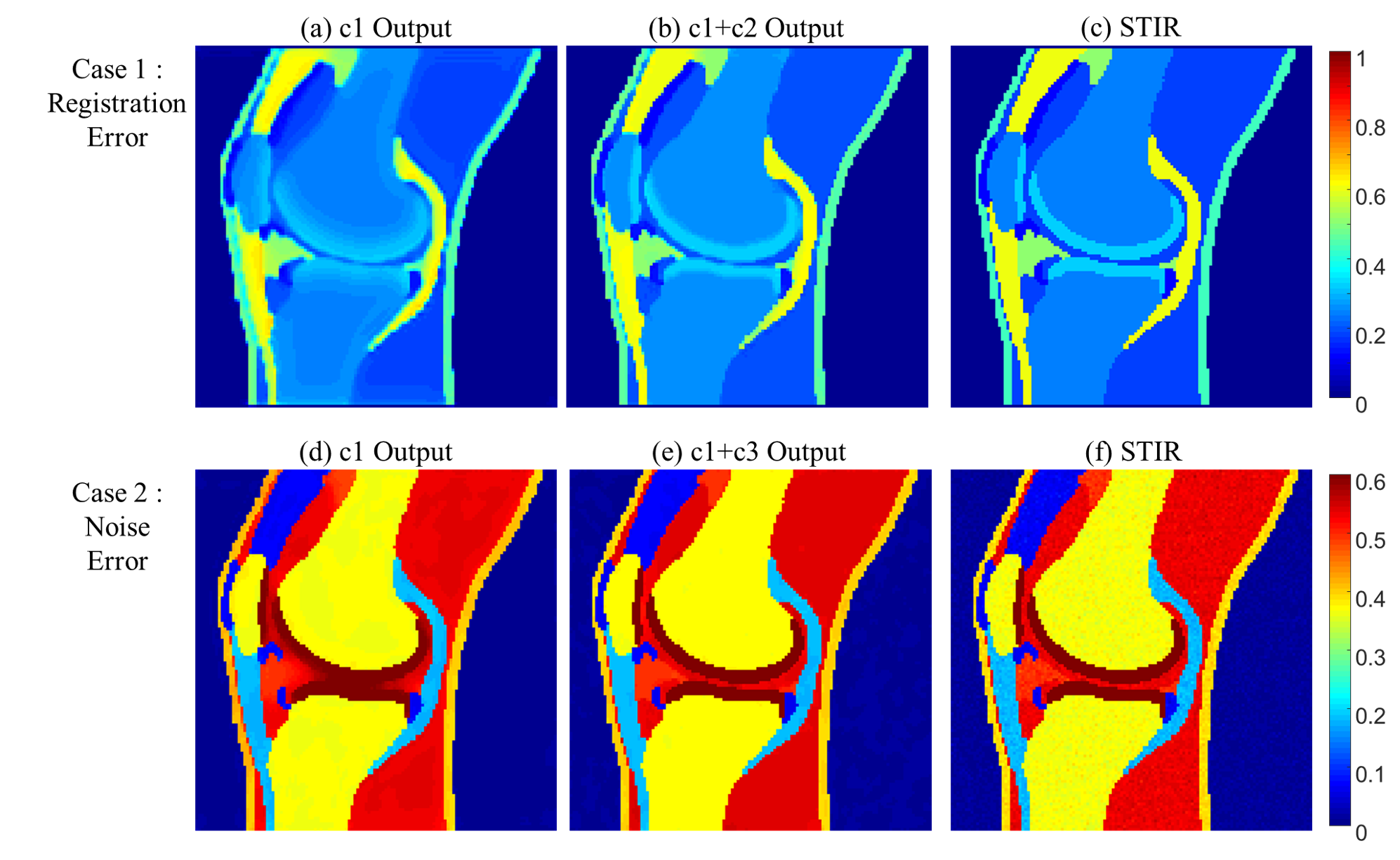
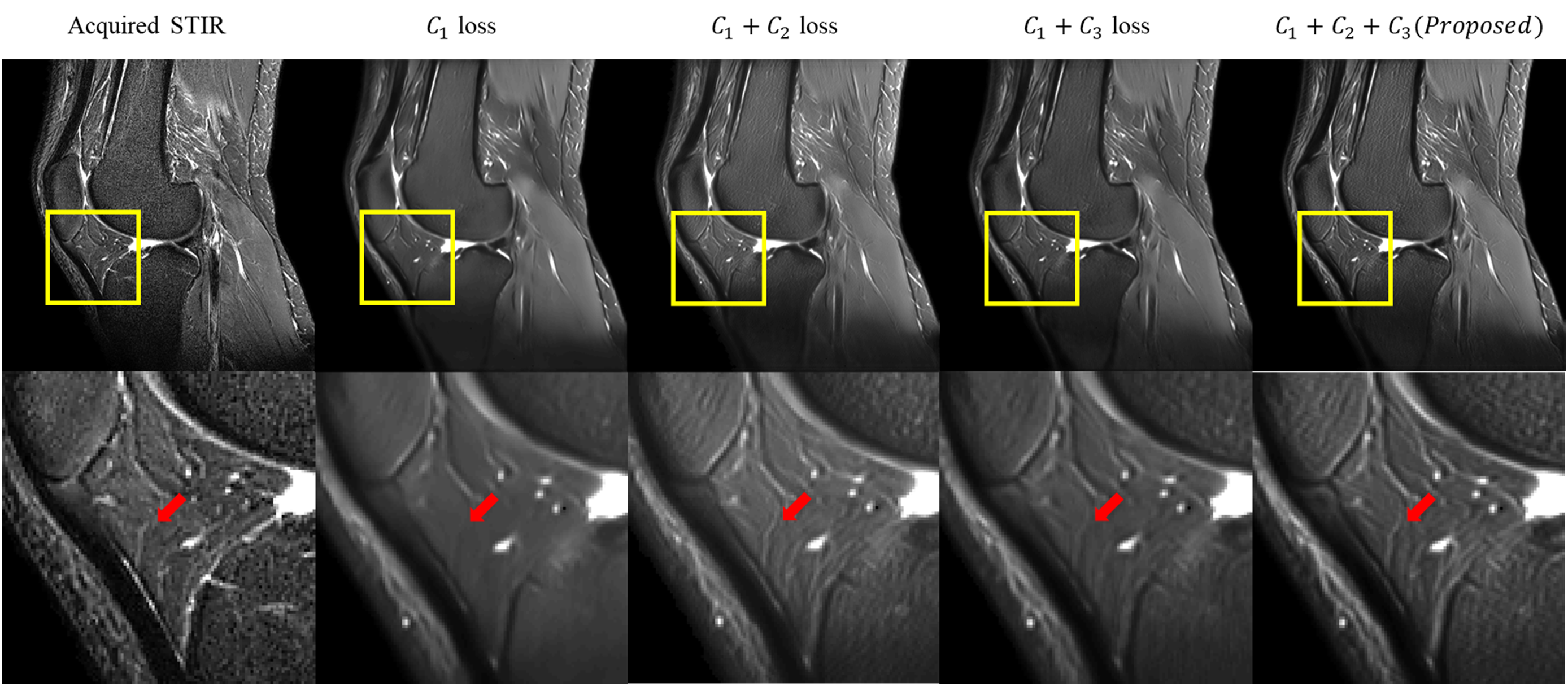
The results of two simulation experiments show the effects of the c2 loss function and the c3 loss function. First, we randomly shifted the multi-contrast images of simulation dataset by 0 to 2 pixels, vertically and horizontally, to show that the c2 loss function corrects misregistration. Figure. 2b and 2c show the results of this experiment when only the c1 loss function is used for training and when the c1 and c2 loss functions are used together, respectively. When only the c1 loss is used, blurring due to misregistration is severely shown. On the other hand, this blurring is corrected and the boundary becomes more clearly distinguished when the c2 loss function is used together. Figure. 2e and 2f show the results of additional noise simulation. When only c1 loss is used for training, the intensity distributions between tissues are unclear and it is hard to distinguish the tissues due to noise. On the other hand, the intensity level difference is clearly distinguished between tissues when c3 loss is used with c1 loss for training. Figure. 3 shows that our proposed loss is applied in-vivo MR image. When all the loss components were used for training, the result image is most similar to the acquired STIR.

Conclusion

This study suggests that our method can generate a STIR image without additional scanning. Our deep-learned STIR images offered a potential alternative to the STIR pulse sequence when additional scanning is limited or STIR artifacts are severe. And our proposed loss shows that improved results for the contrast conversion using multiple images.

Acknowledgements

This research was supported by Basic Science Research Program through the National Research Foundation of Korea(NRF) funded by the Ministry of Science and ICT (2019R1A2B5B01070488), and Bio & Medical Technology Development Program of the National Research Foundation (NRF) funded by the Ministry of Science and ICT (NRF-2018M3A9H6081483)