Introduction

Magnetic resonance imaging (MRI) holds promise to provide imaging biomarkers for a range of diseases and could provide characterisation of changes in the tissue structure of white matter, e.g. loss of myelin or increase in iron storage in deep brain structures. Quantitative susceptibility mapping (QSM) aims to extract the magnetic susceptibility of tissues from MRI phase measurements, which requires the solution of an ill-posed inverse problem. Recently, it has been proposed to solve this problem using deep convolutional neural networks [1, 2, 3]. The current state-of-the-art methods, however, utilize an L2 norm to train the network which leads to over-smooth solutions. Generative Adversarial Networks (GANs [4]) have been employed to increase the performance of such image-to-image translation problems [5] and have been applied recently to the dipole inversion problem in QSM [6]. In this work we aim to train a conditional GAN to learn the mapping from MRI signal phase to QSM, and compare the performance with other QSM methods using the data made available by the QSM challenge 2.0 [8]. The difference with existing methods is the new architecture for the generator, called ResUNet, and that we only utilize simulated data to train the cGAN.

Method

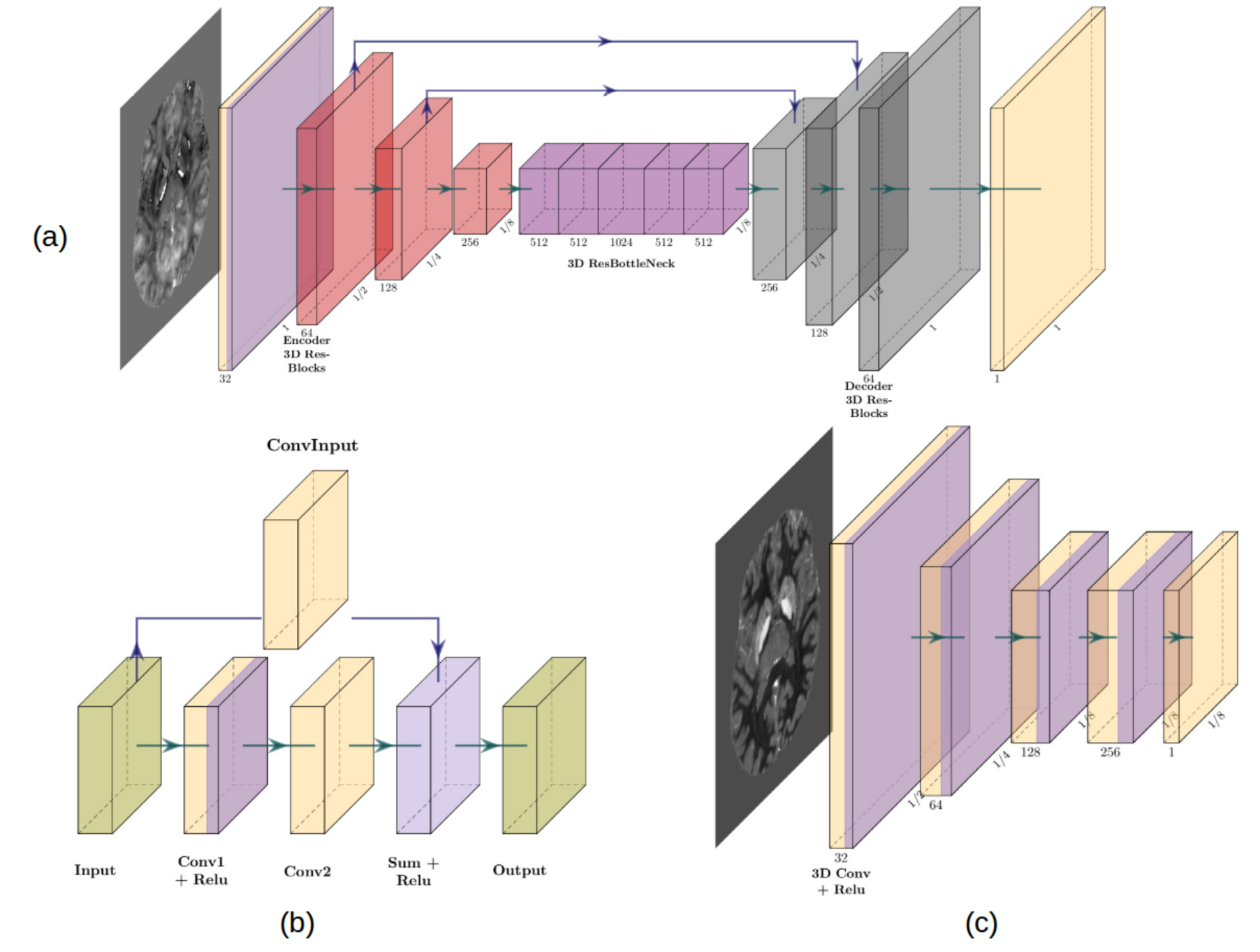
Our GAN architecture (fig.1) is composed of two different networks, a generator (G) and a discriminator (D). G is a deep fully convolutional encoder-decoder architecture with both long and short skip connections. The long connections are concatenations between layers in the encoder and the decoder at the same resolution, while the short connections are achieved using residual blocks [7] between adjacent convolutional layers. These residual connections are used to facilitate the backwards flow of gradients and so to improve the way the network learns. D is a PatchGAN encoder architecture similar to the architecture used in pix2pix [5]. Importantly, in PatchGAN the discriminator D only works at a patch volume of size 8 in order to determine whether the given input is real or fake. It therefore penalizes structures at the scale of patches and can be seen as a loss function that refines the details in the generated volume. As such, PatchGAN enhances small spatial details compared to commonly applied loss functions and the resulting images appear less smooth. The input to D is either a pair of a real input volume conditioned either with its ground truth (x,y) or with a volume created by the Generator (x, G(x,z)). One part of the loss to be optimized is the conditional adversarial loss where G tries to minimize what D is maximizing (equation 1), while the second part is only applied to G that minimizes a standard L1 loss (equation 2) which is multiplied by a weight of 100 such that the generated volume will not differ too much from the ground truth.
$$L_{cGAN} = \mathbb{E}_{x,y}[\log D(x,y)] + \mathbb{E}_{x, z}[\log 1 - D(x,G(x,z))]\qquad(1)$$
$$L_{L1}(G) = \mathbb{E}_{x,y,z}[\| y - G(x,z)\|_{1}]\qquad\qquad\qquad\qquad\quad(2)$$
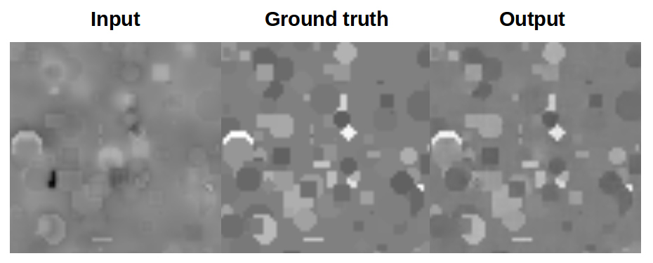
The training is done in an alternating fashion, where the generator has to fool the discriminator by generating volumes that look as close as possible to the reality, whereas the discriminator has to detect whether the volume input has been generated or is a real example. The networks were implemented using Tensorflow 1.13, the Adam optimizer with a learning rate of 1e-4 and beta1 0.5. The network was trained on 25 000 simulated volumes (fig.2) of size 64x64x64 as ground truth with different geometrical shapes whose values match the distribution of a realistic QSM dataset [8]. We then applied the forward model to the simulated magnetic susceptibility distribution to generate the input data for the network. To assess the performance of our approach, we applied the trained network to the dataset provided in [8] and also applied the network to in vivo phase data.

Results

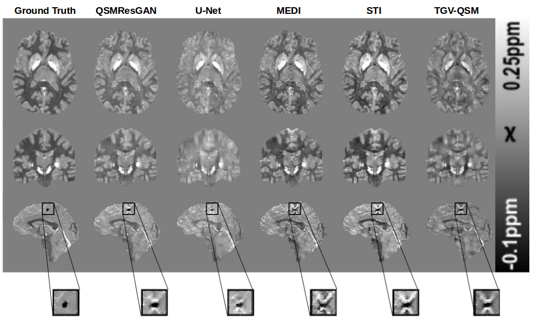
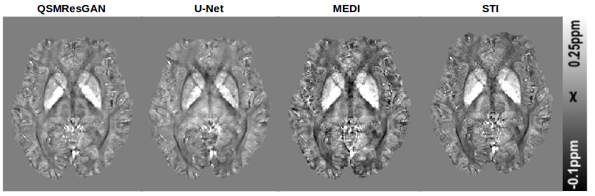
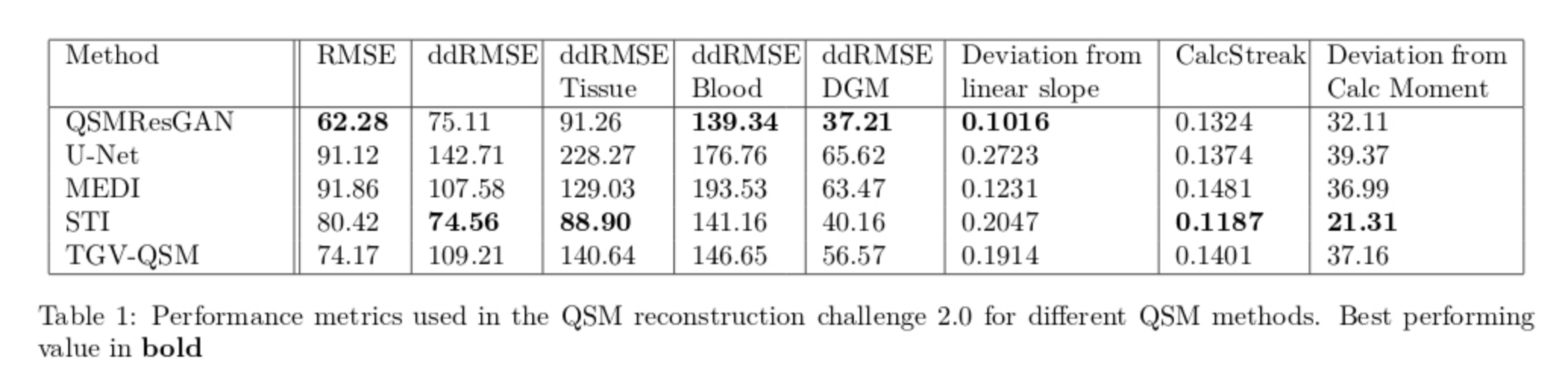
Table 1 shows the metrics for comparing different commonly used methods for QSM. Our network performs best in 4 metrics, on par with STI, which also performs best in 4 (different) metrics. This can also be seen in the visual comparison (fig.3) where our approach shows reduced noise and smoothness, as well as substantially reduced streaking artefacts. Fig.4 shows the comparison of four commonly used QSM methods on in vivo data set, confirming that the approach is applicable to a real world scenario with similar results.

Conclusion

Our proposed conditional generative adversarial network shows a very good performance when judged by the QSM challenge metrics and has improved spatial details and streaking artefact suppression when applied to real world MRI data, while being trained using simulated data. This potentially reduces the need for in vivo and patient data and the risk of over-fitting.

Acknowledgements

The authors acknowledge the facilities and scientific and technical assistance of the National Imaging Facility, a National Collaborative Research Infrastructure Strategy (NCRIS) capability, at the Centre for Advanced Imaging, The University of Queensland. MB acknowledges funding from Australian Research Council Future Fellowship grant FT140100865. This research was undertaken with the assistance of resources and services from the Queensland Cyber Infrastructure Foundation(QCIF). The authors gratefully acknowledge Aiman Al Najjer, Nicole Atcheson, and Anita Burns for acquiring data.