3532
Utility of Stockwell Transform variants for local feature extraction from MR images: evidence from multiple sclerosis lesions
Glen Pridham1, Olayinka Oladosu2, and Yunyan Zhang1
1Department of Radiology, Department of Clinical Neurosciences, Hotchkiss Brain Institute, University of Calgary, Calgary, AB, Canada, 2Department of Neurosciences, Hotchkiss Brain Institute, University of Calgary, Calgary, AB, Canada
1Department of Radiology, Department of Clinical Neurosciences, Hotchkiss Brain Institute, University of Calgary, Calgary, AB, Canada, 2Department of Neurosciences, Hotchkiss Brain Institute, University of Calgary, Calgary, AB, Canada
Synopsis
The Stockwell Transform (ST) is an advanced local spectral feature estimator, that is prohibitively large for use in machine learning applications for typical MR images. We compared two memory-efficient variants: the Polar ST (PST) and the Discrete Orthogonal ST (DOST) as feature extraction steps in competing random forest classifiers, built to classify white matter regions-of-interest as: lesion or normal-appearing. The DOST failed to out-perform guessing, whereas the PST: out-performed guessing, and improved the accuracy of an intensity-based random forest, achieving 88.8% accuracy. We conclude that the PST can complement MR intensity, whereas the DOST may not.
Introduction
The Stockwell Transform1 (ST) is a promising image analysis tool used to extract pixel-wise spectral features, however, the standard procedure is computationally prohibitive. This necessitates the use of memory-efficient variants, such as the Polar Stockwell Transform2,3 (PST), or the Discrete Orthogonal Stockwell Transform4 (DOST). Texture analyses using the PST have succeeded in differentiating lesion pathology5-7 and brain tissue types2 in multiple sclerosis (MS), based on MR imaging (MRI). The DOST is a more efficient variant, and has shown utility for texture classification8, however, it has not been tested for localized feature extraction. In this study, we compared the DOST, polar-indexed DOST (PDOST), PST, and rotationally-invariant radial PST (RPST) for their use in differentiating MS lesions in brain white matter from contralateral normal appearing white matter (NAWM) as seen in MRI, using a random forest (RF) classifier9. Finally, we tested if successful performing feature set(s) could enhance children RF classifiers based on the MR intensity information.Materials and Methods
ImagingWe used brain MRI scans from 6 MS patients (1 hold-out, 5 cross-validated) recruited for an ongoing clinical study. Institutional approval and informed consent for each patient were obtained. Imaging included: T1-weighted, T2-weighted, and FLAIR MRI acquired on a 3T scanner (Fig. 1). Parameters for T1, T2 and FLAIR were, respectively: TR/TE = 8.2/3.192 ms, 6694/104.96 ms, and 7000/132.508 ms, slice thickness = 1 mm, 3 mm, and 1 mm, matrix size = 256x256, 512x512 and 512x512, and pixel size = 0.9766x0.9766 mm2, 0.4297x0.4297 mm2, and 0.4688x0.4688 mm2. Preprocessing used FSL10,11 for: rigid-body co-registration12,13 to T1, and brain extraction14; then ANTsR for N4 field bias correction15, and finally intensity standardization by dividing by the histogram mode.
Feature Extraction
The FLAIR images were used to calculate pixel-wise features using the PST, DOST and PDOST. The (x,y) coordinates were also included (except for the RPST set).
PST
Consider an image $$$I(x,y)$$$, we used the PST defined by2:
$$P(n,m,k\neq0,\theta) = \sum_i\sum_j\frac{1}{M_{k\theta}(i,j)}\frac{4\pi{}N^2}{(i^2+j^2)}\Big| F^{-1}\Big(e^{-\frac{2\pi^2(\alpha^2+\beta^2)}{k^2}}F(I)(\alpha+i,\beta+j)\Big)\Big|^2 \qquad\text{(1)}\\
P(n,m,k=0,\theta) = F(I)(0,0) $$
where $$$(\alpha,\beta)$$$ are the Cartesian Fourier indices, $$$k=\text{round}(\sqrt{\alpha^2+\beta^2})$$$, $$$\theta=\text{round}(\arctan{(\beta/\alpha)})$$$, $$$F$$$ is the Fourier transform, and $$$M_{k\theta}$$$ is the frequency of the polar indices $$$(k,\theta)$$$. The PST was an intermediate step in calculating the RPST, $$$R$$$, and the angular PST, $$$A_{\Delta{}k_0}$$$:
$$R(n,m,k)=\frac{1}{N_\theta}\sum_\theta{}P(n,m,k,\theta)\\
A_{\Delta{}k_0}(n,m,\theta)=\frac{1}{N_k}\sum_{k=k_0}^{k_0+\Delta{}k_0}P(n,m,k,\theta)$$
where $$$N_k$$$ and $$$N_\theta$$$ are the number of radial frequencies and angles, respectively, and $$$\Delta{}k_0$$$ is a user-defined frequency band2.
DOST
The 1D-DOST uses the inner product of an input signal with orthogonal basis functions of the form4:
$$\Phi_{\nu,\tau}(k) \equiv \frac{ie^{-i\pi\tau}}{\sqrt{\beta}}\frac{e^{-2\pi{}i(\frac{k}{N}-\frac{\tau}{\beta})(\nu-\frac{\beta}{2}-\frac{1}{2})}-e^{-2\pi{}i(\frac{k}{N}-\frac{\tau}{\beta})(\nu+\frac{\beta}{2}-\frac{1}{2})}}{2\sin{(\pi(\frac{k}{N}-\frac{\tau}{\beta}))}}$$
where $$$\beta=2\nu/3$$$, $$$\nu$$$ is the central frequency, and $$$\tau$$$ is the time index. We used the symmetric DOST rules for selecting $$$(\nu,\tau)$$$16. We calculated the 2D-DOST of an image using the 1D-DOST across all columns, then all rows.
PDOST
We defined the PDOST here in the same way as the PST, but substituting the DOST modulus for the ST in (1).
Classification
White matter regions of interest (ROIs) for: lesions and contralateral normal-appearing control, were semi-automatically identified on T1/FLAIR using the Lesion Growth Algorithm17 with manual corrections. The PST, DOST and PDOST features were used to train a set of random forests to classify ROIs as lesion vs control. Significantly accurate classifiers were selected as parents to new random forests that included as features: MR intensity information, and the parent prediction. Accuracy measures were estimated by 10-fold, 10-repeat cross-validation18 (mean $$$\pm$$$ sd). Pearson’s $$$\chi^2$$$ test19 was used to compare classifier performance to a guess.
Results
Both the PST and the RPST feature sets succeeded, whereas the DOST and PDOST failed, to perform significantly better than guessing (Table 1). Investigating, we observed that the RPST appeared to detect: anatomical boundaries, such as ventricles (Fig. 2B-D, Fig. 3B), and lesion size (Fig. 3A). The pixel-wise classification performance of the training dataset was qualitatively assessed using a slice from the hold-out patient (Fig. 3B-C). Features from T2 showed similar results.Using children classifiers, the PST improved the classification accuracy over the FLAIR intensity alone (Wilcox $$$p = 1.7\cdot10^{-4}$$$); more accurate than FLAIR+PST was FLAIR+RPST (Wilcox $$$p = 3.8\cdot10^{-3}$$$). We combined the: RPST parent classifier prediction, T1, T2 and FLAIR, to generate a maximally accurate classifier. Table 2 summarizes.
Discussion
Classification accuracies suggest that the PST succeeded due to the RPST, consistent with previous studies2,5-7. The RPST was observed to learn the location of ventricle boundaries, a region where MS lesions are likely to occur20, and lesion size, whereas the DOST failed to perform better than a guess, ostensibly due to its sparsity/lack of resolution. Furthermore, the RPST provided additional information to complement MR intensities. Relative to existing approaches21, the RPST classifiers performed poorly without intensity information, but performed well with it.Conclusion
We observed that the PST succeeded in extracting lesion-sensitive features from brain MRI scans of MS patients, in contrast to the DOST. The PST appears to detect ventricle boundaries and size information, which enhances lesion detection over MR intensity alone.Acknowledgements
We thank the patient volunteers for participating in this study and the funding agencies for supporting the research including the Natural Sciences and Engineering Council of Canada (NSERC), Multiple Sclerosis Society of Canada, Alberta Innovates, Campus Alberta Neuroscience-MS Collaborations, and the HBI Brain and Mental Health MS Team, University of Calgary, Canada.References
- Stockwell R, Mansinha L, Lowe R. Localization of the complex spectrum: the S transform. IEEE Trans Signal Process. 1996;44(4):998-1001.
- Pridham G, Steenwijk M, Geurts J, Zhang Y. A discrete polar Stockwell transform for enhanced characterization of tissue structure using MRI. Magn Reson Med. 2018;80(6):2731-2743.
- Zhou Y. Boundary detection in petrographic images and applications of S-transform space-wavenumber analysis to image processing for texture definition [PhD Thesis]. London, Ontario: University of Western Ontario; 2002.
- Stockwell R. A basis for efficient representation of the S-transform. Digital Signal Process. 2007;17(1):371-393.
- Zhang Y, Zhu H, Metz L, Mitchell J. A new MRI texture measure to quantify MS lesion progression. In 12th ISMRM proceedings. Kyoto, Japan. 2004.
- Zhang Y, Zhu H, Mitchell J, Costello F, Metz L. T2 MRI texture analysis is a sensitive measure of tissue injury and recovery resulting from acute inflammatory lesions in multiple sclerosis. Neuroimage 2009;47(1):107-111.
- Zhang Y, Jonkman L, Klauser A, Barkhof F, Yong V, Metz L, Geurts J. Multi-scale MRI spectrum detects differences in myelin integrity between MS lesion types. Mult Scler J 2016;22(12):1569-1577.
- Drabycz S, Stockwell RG, Mitchell JR. Image texture characterization using the discrete orthonormal S-transform. J Digit Imaging. 2009;22:696-708.
- Liaw A, Wiener M. Classification and Regression by randomForest. R News. 2002;2(3):18-22.
- Jenkinson M, Beckmann CF, Behrens TE, Woolrich MW, Smith SM. FSL. Neuroimage. 2012;62(2):782-790.
- Muschelli J, Sweeney E, Lindquist M, Crainiceanu C. fslr: Connecting the FSL Software with R. R J. 2015;7(1):163-175.
- Jenkinson M, Smith SM. A global optimisation method for robust affine registration of brain images. Med Image Anal. 2001;5(2):143-156.
- Jenkinson M, Bannister PR, Brady JM, Smith SM. Improved optimisation for the robust and accurate linear registration and motion correction of brain images. Neuroimage. 2002;17(2):825-841.
- Smith SM. Fast robust automated brain extraction. Hum Brain Mapp. 2002;17(3):143-155.
- Avants BB. ANTsR: ANTs in R: Quantification Tools for Biomedical Images. R Package v 0.4.8. 2019.
- Wang Y, Orchard J. Fast discrete orthonormal Stockwell transform. SIAM J Sci Comput. 2009;31(5):4000-4012.
- Schmidt P, Gaser C, Arsic M, Buck D, Förschler A, Berthele A, Hoshi M, Ilg R, Schmid VJ, Zimmer C, Hemmer B. An automated tool for detection of FLAIR-hyperintense white-matter lesions in multiple sclerosis. Neuroimage. 2012;59(4):3774-3783.
- Kuhn M, et al. caret: Classification and Regression Training. R Package v 6.0-84. 2019.
- R Core Team (2019). R: A language and environment for statistical computing. R Foundation for Statistical Computing, Vienna, Austria. https://www.R-project.org/.
- Harmouche R, Collins L, Arnold D, Francis S, Arbel T. Bayesian MS lesion classification modeling regional and local spatial information. In 18th ICPR proceedings. Hong Kong, China: IEEE; 2006.
-
Lladó
X, Oliver A, Cabezas M, Freixenet J, Vilanova J, Quiles A, Valls L,
Ramió-Torrentà L, Rovira À. Segmentation of multiple sclerosis lesions in brain
MRI: a review of automated approaches. Inf Sci. 2012;186(1):164-185.
Figures
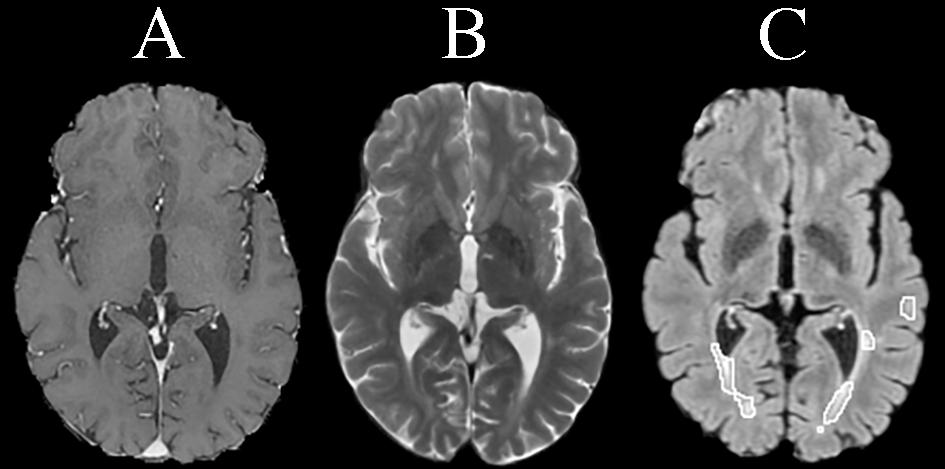
Fig. 1. Sample slice from dataset (holdout patient). A: T1, B:
T2, C: FLAIR with lesion mask outlined.
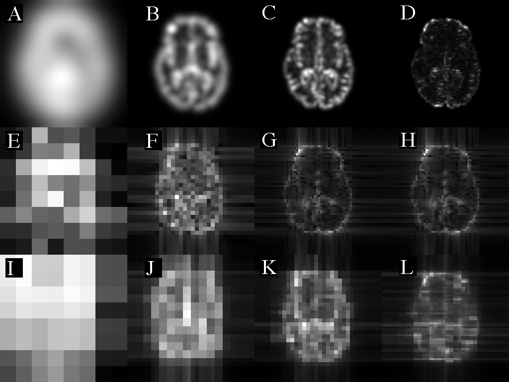
Fig. 2. Example radial spectrum images. Images are: PST (A-D),
DOST (E-H) and PDOST (I-L) for frequencies: 8/256 (A,E,I), 32/256 (B,F,J), 64/256
(C,G,K) and 128/256 /pixel (D,H,L), all on modulus scale.
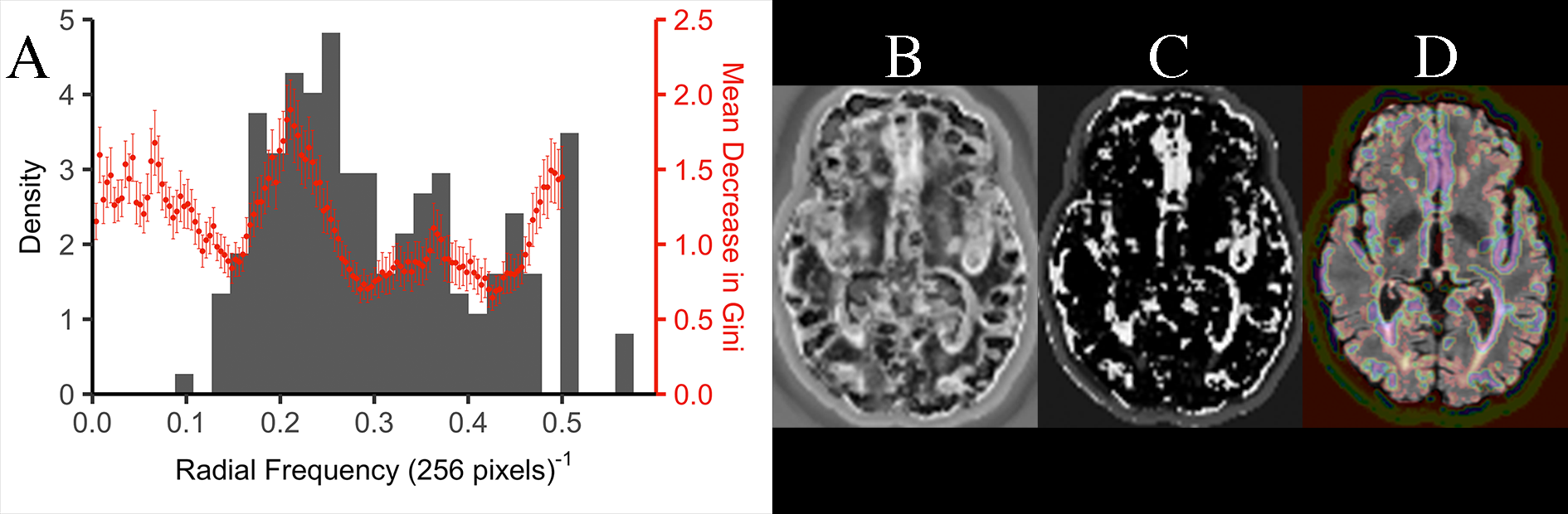
Fig.
3. RPST classifier observations. (A): feature
importance (red) correlates with lesion inverse diameter histogram (grey). Also
shown is the lesion classification probability for (brighter = more likely a lesion):
RPST classifier (B), and RPST+FLAIR+T1+T2 classifier (C). In (D) the image (C) has
been super-imposed onto the original FLAIR (red-purple = low-high lesion
probability).
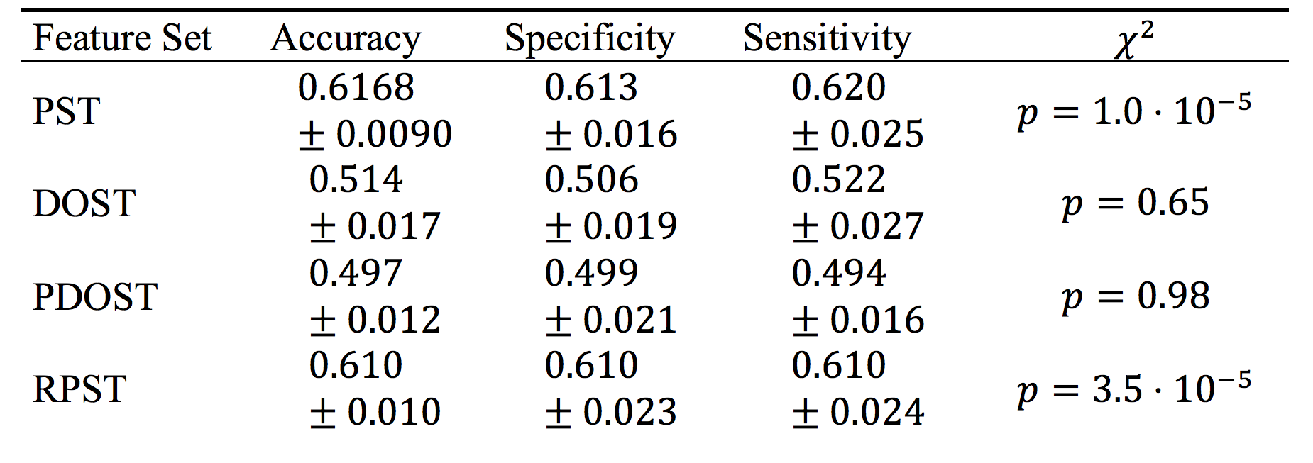
Table 1. Parent classifiers performance summary.
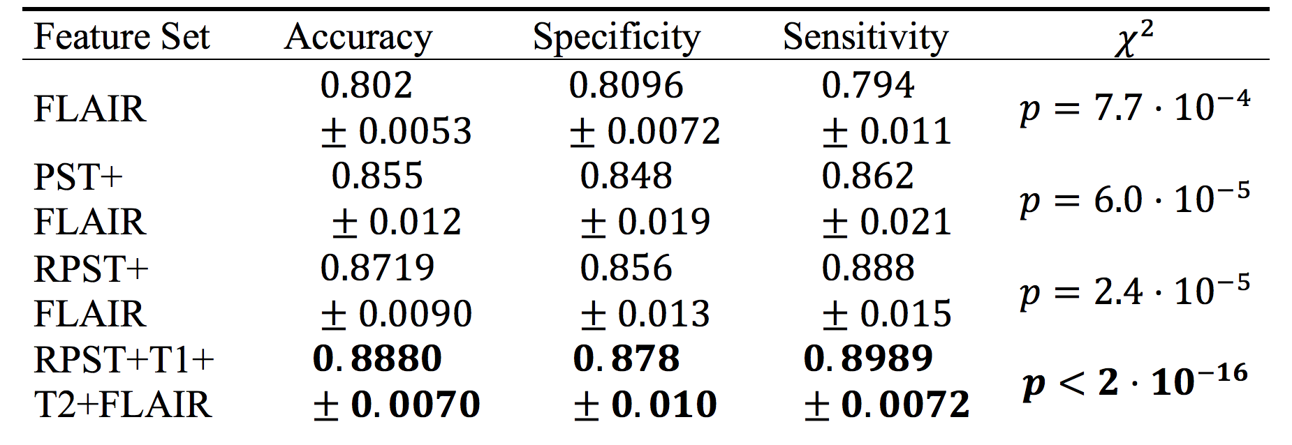
Table 2. Children classifiers performance summary.