Introduction

Traditionally, MR images are first reconstructed from k-space data, after which pathology detection and characterization are performed in the image domain. At present, emerging deep learning techniques and rapidly expanding computational power offer the unprecedented opportunity to revolutionize the MRI reconstruction¹ and diagnosis. In this study, we propose a new strategy for automatic pathology detection and classification (tumor presence, tumor sizes and locations) directly from k-space data through deep learning. This approach presents an alternative MR diagnostic paradigm that may lead to new tools for automatic and effective pathology screening, detection and characterization.

Method

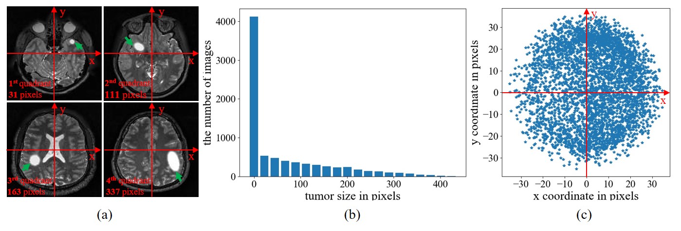
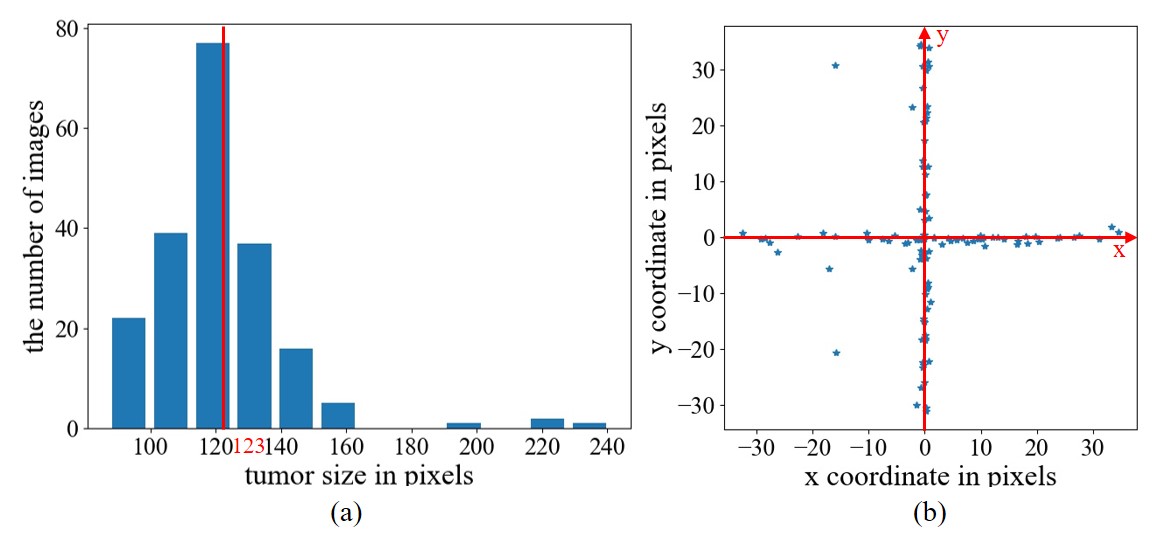
Data Preparation
WU-Minn HCP database² was used, where T2-weighted images were acquired using 3D SPACE with isotropic resolution of 0.7 mm. In this study, the datasets were prepared as follows: (1) magnitude images from 450 normal subjects were first selected from HCP database; (2) 90 images from the central consecutive slice locations were extracted from each of these 450 3D image volumes , B1 corrected, and resized to 128×128; (3) these 450 90-slice image datasets were randomly divided for training (315 or 70%), validation (45 or 10%) and testing (90 or 20%); (4) 315 training image datasets were augmented four times to 1260 datasets by small 2D in-plane image translations/dilations/contractions; (5) random and smooth 2D 2nd-order phase variations were added to these magnitude images to create realistic and fully sampled k-space data; and (6) simulated tumors were added to 50% of these images with random location, size, shape and brightness. In brief, the tumor was synthesized by changing the signal intensity within an ellipse, with its short and long axis varying between 3.5% and 20% of the FOV. Its peak intensity was set to that of cerebrospinal fluid (CSF). The simulated tumor edges were then blurred with Gaussian smoothing to minimize distinct ringing in k-space. All tumors were classified into two categories by size (larger or smaller than 123 pixels, which is the median value ranging from 0 to 438 pixels) and four quadrants by location based on the tumor center. Samples of simulated tumors were shown in Figure 1(a). The size and location distribution of simulated tumors were shown in Figures 1(b) and 1(c), respectively.

CNN Model
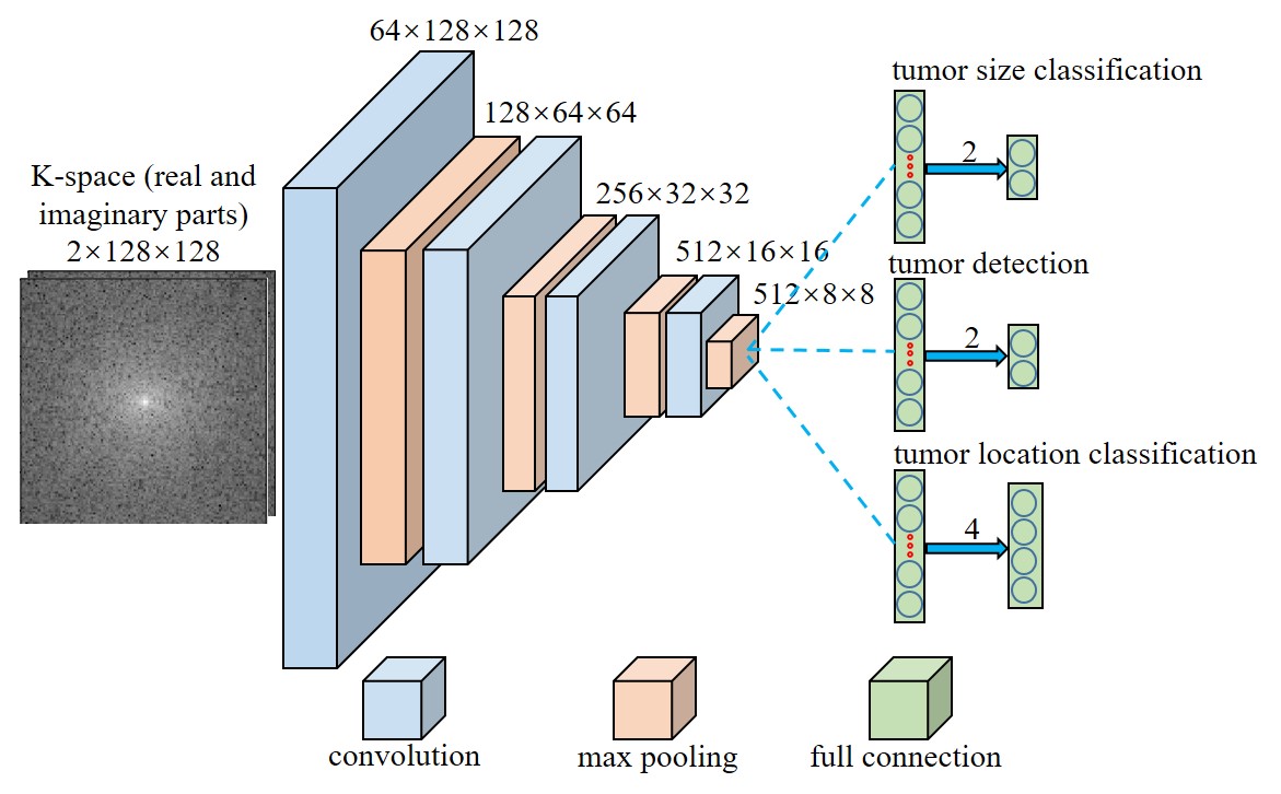
As illustrated in Figure 2, a convolutional neural network (CNN) architecture was designed for tumor detection and tumor sizes/locations classification. Three models share the layers that are composed by convolutional and maxpooling layers. Each convolutional layer is followed by a batch normalization layer and each maxpooling layer is followed by a rectified linear unit (ReLU) layer. In addition, each model has its own fully connected layer for classification. The model was trained using 113,400 images with 50% tumor occurrence rate per image. Validation and testing were performed with 4050 and 8100 images, respectively. The model was designed with Python based on PyTorch 1.0 and implemented on a Linux workstation with two NVIDIA GTX 1080ti GPUs.

Results

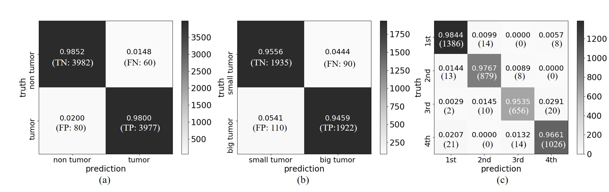
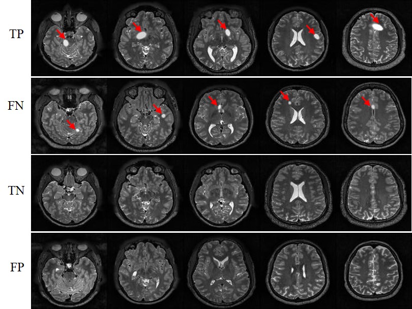
Figure 3 presents the outcome matrices of our proposed pathology detection and classification results. Our approach yielded generally high sensitivities and specificities, demonstrating the capability of the proposed strategy for image-free tumor detection and tumor sizes/locations classification directly from k-space data. The confidence interval for tumor detection, tumor size and location classification under confidence 99% is 98.23±0.37%, 95.07±0.62% and 97.27±0.47%, respectively. The false negative rate for tumor detection was 1.5% and they mostly correspond to small tumors. The false positive rate was 2.0% and they mostly occurred for structures that might be similar to simulated tumors, e.g., CSF. Example images with true positive (TP), false negative (FN), true negative (TN) and false positive (FP) tumor detection outcomes are shown in Figure 4. Figure 5 shows the distribution of failed cases of tumor sizes/locations classification, which occurred mostly near the size and location classification boundaries.

Discussion and conclusions

This study demonstrates a new MR diagnostic paradigm where pathology detection and characterization can be performed directly from MR k-space data and bypass the process of image reconstruction. Although results are highly promising, further studies are warranted to advance this conceptually new approach for image-free pathology detection and classification: (1) model improvement, including the refinement of tumor classifications schemes, incorporation of 3D tumor within multi-slice image datasets, and consideration of multi-channel k-space data; (2) use of images covering specific anatomic regions to train the model to detect pathology in these specific regions; (3) use of more realistic pathology or tumor models³ and incorporation of clinical tumor images through transfer learning⁴; and (4) comparison with the traditional image-domain pathology detection/classification to explore the true advantages of our k-space approach, e.g., robust tumor detection from extremely sparse k-space for fast and image-free pathology screening. In summary, our proposed approach presents an alternative MR diagnostic paradigm that may lead to potentially more powerful tools for efficient and effective pathology screening, detection and characterization

Acknowledgements

This study is supported in part by Hong Kong Research Grant Council (C7048-16G and HKU17115116 to E.X.W. and HKU17103819 to A.T.L.), Guangdong Key Technologies for Treatment of Brain Disorders (2018B030332001) and Guangdong Key Technologies for Alzheimer's Disease Diagnosis and Treatment (2018B030336001) to E.X.W. We thank Karim El Hallaoui and Anson Leung for their technical contributions.