Introduction

There have been significant advances in the development and use of deep learning algorithms for disease classification, such as those based on convolutional neural networks (CNNs). However, the ability to interpret deep learning models has lagged considerably behind. Recently several studies have shown the potential of a heatmap generation method, class activation mapping (CAM)1, to highlight the most critical imaging feature patterns detected by a CNN classification model. More recently, 2 new updates of CAM that have increasing generalizability have emerged, named gradient (Grad)-CAM2, and Grad-CAM ++3 respectively. In this study, our goal was to compare the utility of the 3 CAM-related methods based on 8 deep learning models from 5 CNN algorithms. The models were trained for classifying brain MRI into 3 categories: relapsing-remitting multiple sclerosis (RRMS), secondary progressive MS (SPMS), or healthy control.

Methods

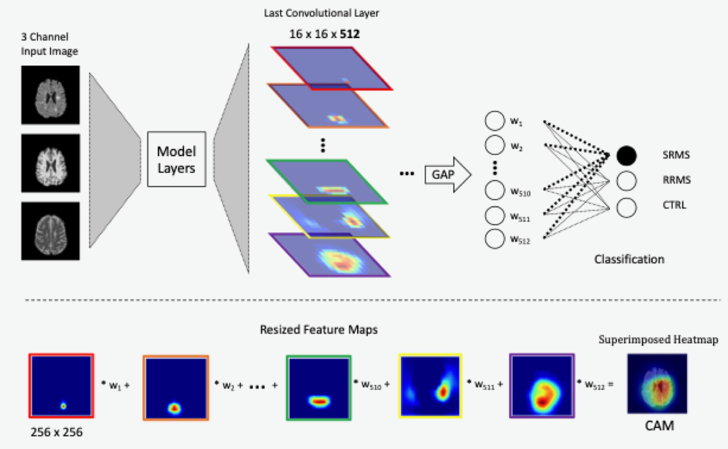
The CNN algorithms included: AlexNet, ResNet50, ResNet18, VGG16, and VGG 19. We applied transfer learning and imported the ImageNet weights for each model trained initially for classifying 1000-class natural images. The networks were then modified to generate 3 output classes: RRMS, SPMS, and controls, based on 3-channel inputs from T1-, T2-weighted, and FLAIR MRI. Our dataset included MRI scans from 19 MS patients (10 RRMS and 9 SPMS) and 19 age- and sex-matched controls. To standardize the scans, we co-registered T2 and FLAIR to T1 MRI following image non-uniformity correction, such that each pulse sequence contained 156 MRI slices, which were reduced to 135 to improve computation efficiency by removing slices not containing significant brain regions. Subsequently, all images underwent histogram equalization, followed by rotation, translation, and scaling for data augmentation during training. Dataset splitting included 75%, 10%, and 15% for training, validation, and testing purposes.
The CAM calculation required the addition of a global average pooling (GAP) layer to the CNN models. This allowed direct multiplications between the same number of image feature maps (𝑨𝒌) and their corresponding weights (𝒘𝒄), which relied on the last convolutional layer of a CNN. Summation of the multiplications generated CAM using equation: 𝑳𝒄 = ∑ 𝒘𝒄 𝑨𝒌 (Fig. 1). The computation of Grad-CAM and Grad-CAM++ were similar to that of CAM, except that both could work with any convolutional layer of a network. In addition, the weights were generated from the gradient or exponential function of the classification score based on feature maps of the selected layer for Grad-CAM and Grad-CAM++ respectively. To ensure consistency, we used the last convolution layer for both advanced CAM versions, equivalent to CAM. The models from each algorithm except AlexNet and ResNet included two versions: with a GAP or fully connected (FC)/dense layer.
We applied Grad-CAM to all models for heatmap comparison based on their accuracy and loss in image classification, and then added CAM and Grad-CAM++ to the top two ranked models. Other validation metrics included the probability of classification, and consistency and frequency of highlighted areas in brain MRI. All analyses used the Keras deep learning framework and TensorFlow backend, with Tesla K40m and V100 GPUs.

Results

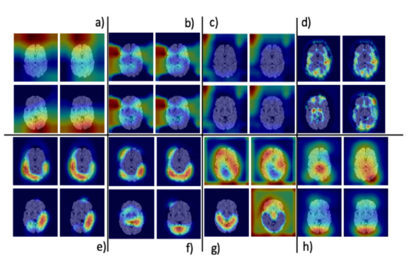
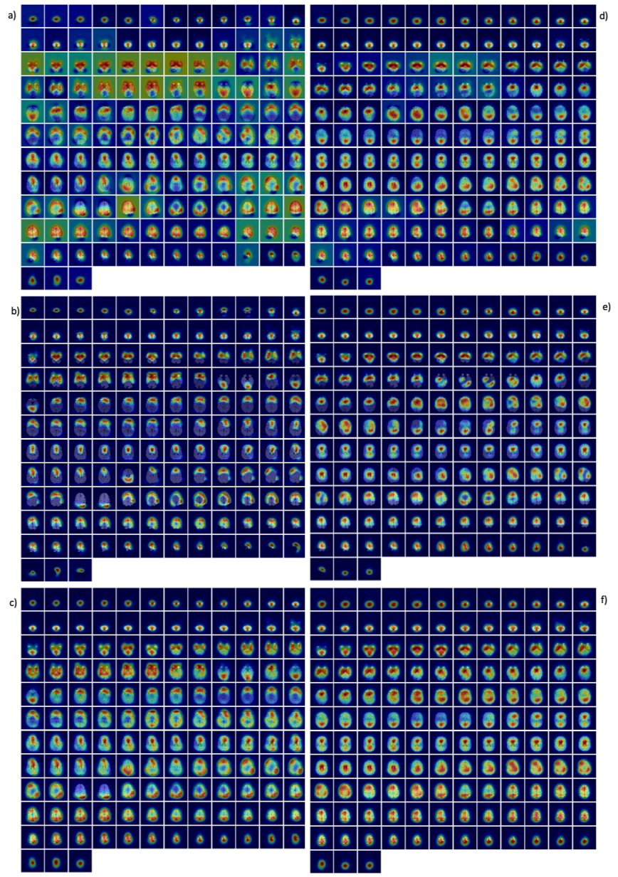
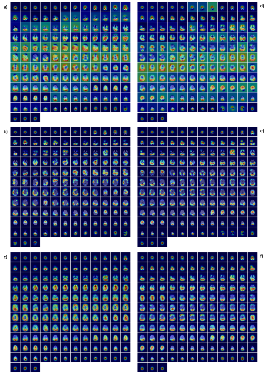
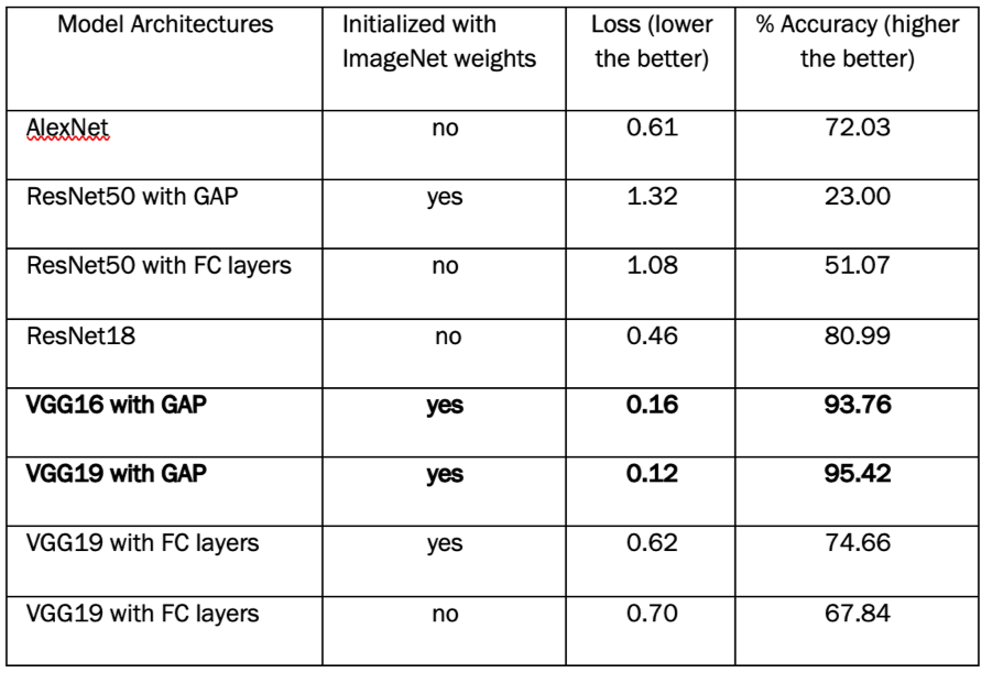
VGG16 with GAP and VGG19 with GAP had the best loss and accuracy (Table 1). From heatmap generation analysis, they both also showed the highest consistency in the patterns of feature highlights, particularly VGG19. Specifically, these models highlighted distinct regions of activation in the brain, with focuses on the frontal (upper) or occipital (lower) lobe, or both in different MRI slices. AlexNet highlighted primarily the background (red regions), and ResNet18 highlighted mostly edges and corners. ResNet50 models almost always highlighted the same area regardless of input image properties, which had the worst outcomes (Fig. 2).
Between subject groups, both VGG16 and VGG19 with GAP showed different highlight patterns. With VGG16, the highlights focused on either frontal or temporal (middle) regions of the brain in SPMS, versus frontal and occipital regions, or only the latter in RRMS. In control subjects, the highlights were mostly in the middle regions. With VGG19, the highlights were similar to VGG16 except in SPMS, which focused on either frontal and occipital regions, or just temporal areas (Figs 3 & 4).
The heatmaps from CAM appeared very similar to Grad-CAM. However, comparing to Grad-CAM, the GradCAM++ heatmap areas were diffuse, with increased background highlights but without significant patterns detected.

Discussion

This study implemented 3 new heatmap generation techniques based on 8 established CNN classification models. We found that classification models with higher accuracy and lower loss had better heatmap patterns for human interpretation. Based on VGG16 and VGG19, Grad-CAM (and CAM) highlighted brain regions that are known to play critical roles in the pathogenesis of MS4 and that were dramatically different between SPMS and RRMS. This may provide novel evidence for understanding the mechanisms of disease development in MS or similar disorders, and discovering new biomarkers for monitoring disease and treatment. GradCAM++ showed better generalization results but that also made it difficult for pattern detection.

Conclusion

Advanced interpretation of deep learning models will be critical for improving our ability in bridging deep-learned MRI features to brain pathophysiology and function.

Acknowledgements

We thank the patient and control volunteers for participating this study and the funding agencies for supporting the research including the Natural Sciences and Engineering Council of Canada (NSERC), Multiple Sclerosis Society of Canada, Alberta Innovates, Campus Alberta Neuroscience-MS Collaborations, and the HBI Brain and Mental Health MS Team, University of Calgary, Canada.