Introduction

While tissue phase mapping (TPM) provides a means to quantify regional biventricular three-directional myocardial velocities(1), it is rarely used in clinical practice due to labor intensive manual segmentation of cardiac contours for all time frames. The low signal to noise ratio (SNR) of TPM images makes it challenging to apply automated segmentation methods, especially the right ventricle (RV) that has thinner wall than left ventricle (LV). In this study, we sought to develop a fully automated segmentation method for TPM images using deep learning (DL) and explore different U-Net network architectures combining magnitude and phase images.

Methods

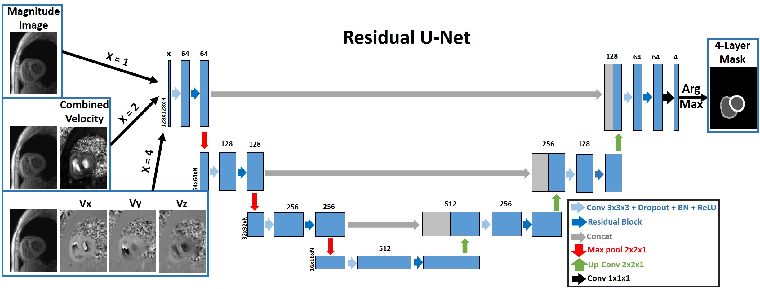
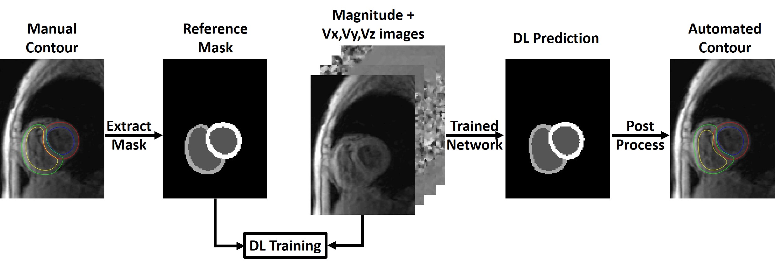
Human Subject & Pulse Sequence: The study included 26 patients (mean age 55.0 ± 12.1 years; 10 males; 16 females) with pulmonary hypertension and 8 healthy controls (mean age 57.8 ± 15.3 years; 4 males; 4 females). All subjects underwent cardiac MRI at 1.5T (MAGNETOM Aera, Siemens) including k-t accelerated TPM using a prospectively ECG-gated, black-blood prepared gradient echo sequence with three-directional velocity encoding(2-5). Time resolved TPM images were acquired for three shot-axis slices at basal, mid-ventricular and apical locations for each subject. In total 97 2D + time TPM slices were used in this study, excluding 5 basal slices that didn’t include RV.
Image Processing: The manual segmentation and data analysis were performed using a custom software package developed in MATLAB by one reader with 2 years of experience as a medical research fellow. As shown in Figure 1, the TPM images and reference masks extracted from manual contours were used as input and reference to train three different DL networks: 1) 1-channel network, which used the magnitude image alone as input; 2) 2-channel network, which used the magnitude image and the combined velocity (V_sum = Sqrt(V_x²+V_y²+V_z²) ) image as input channels; 3) 4-channel network, which used the magnitude image and three dimensional velocity (Vx, Vy, Vz) images as input channels. We used at total of 2,445 manually annotated 2D TPM images (24 subjects, 18 patients and 6 controls, 67 slices, 26-52 time frames per slice) for training and the remaining 1,152 manually annotated 2D TPM images (10 subjects, 8 patients and 2 controls, 30 slices, 31-50 time frames per slice) for testing. We used 3D convolution to process the data slice by slice (2D+time), while the 2D pooling (2x2x1) allows arbitrary number of time frames. For testing, we converted the DL masks to contours by applying automated post-processing in MATLAB and fed the contours to the custom software package for data analysis.
Quantitative Analysis: For different networks, we calculated the Sørensen–Dice index of LV and RV myocardium with manual contoured masks as reference. The TPM data analysis workflow followed previous work (2) comparing 4-channel network deep learning contours with the manual contours.

Results

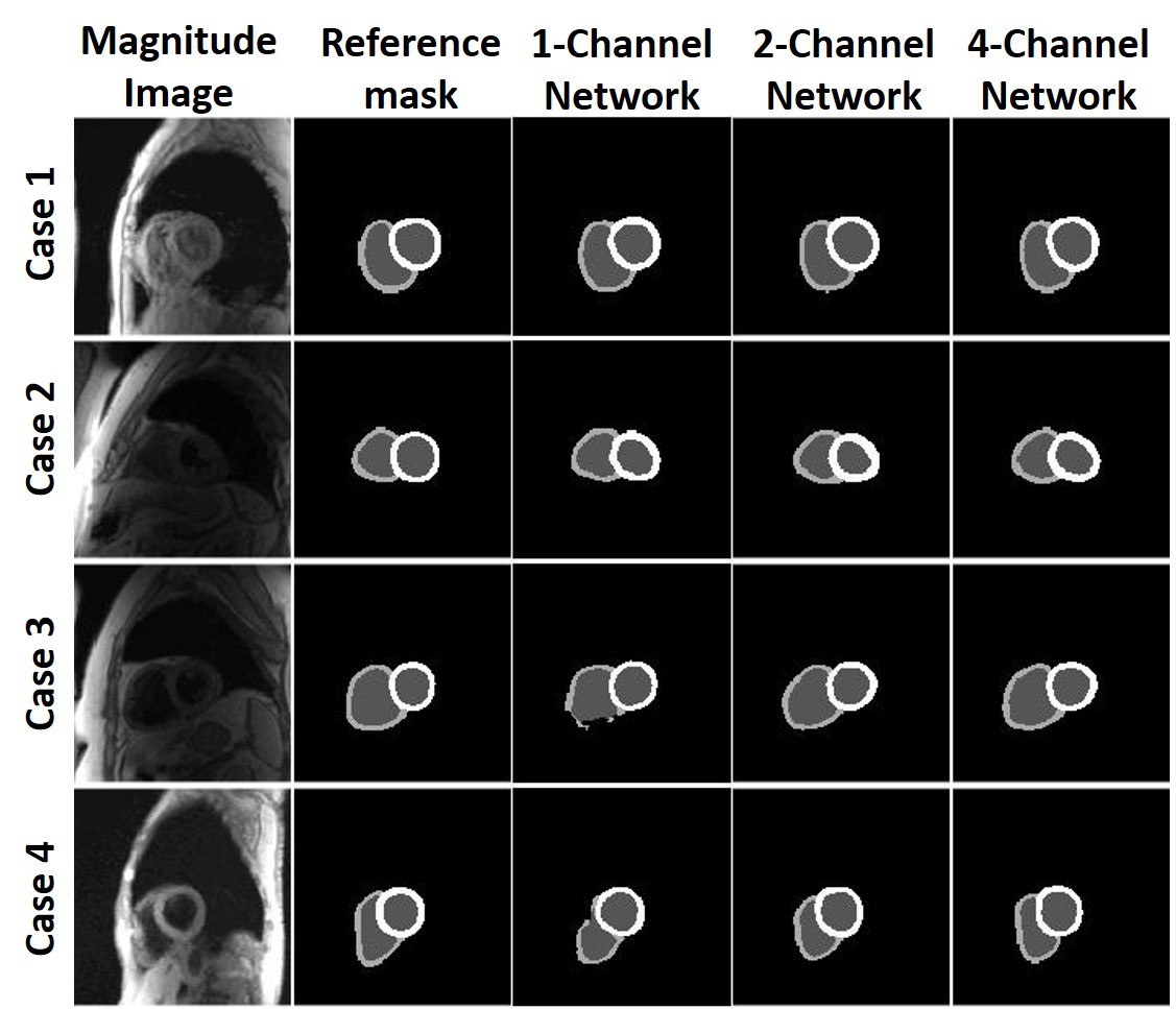
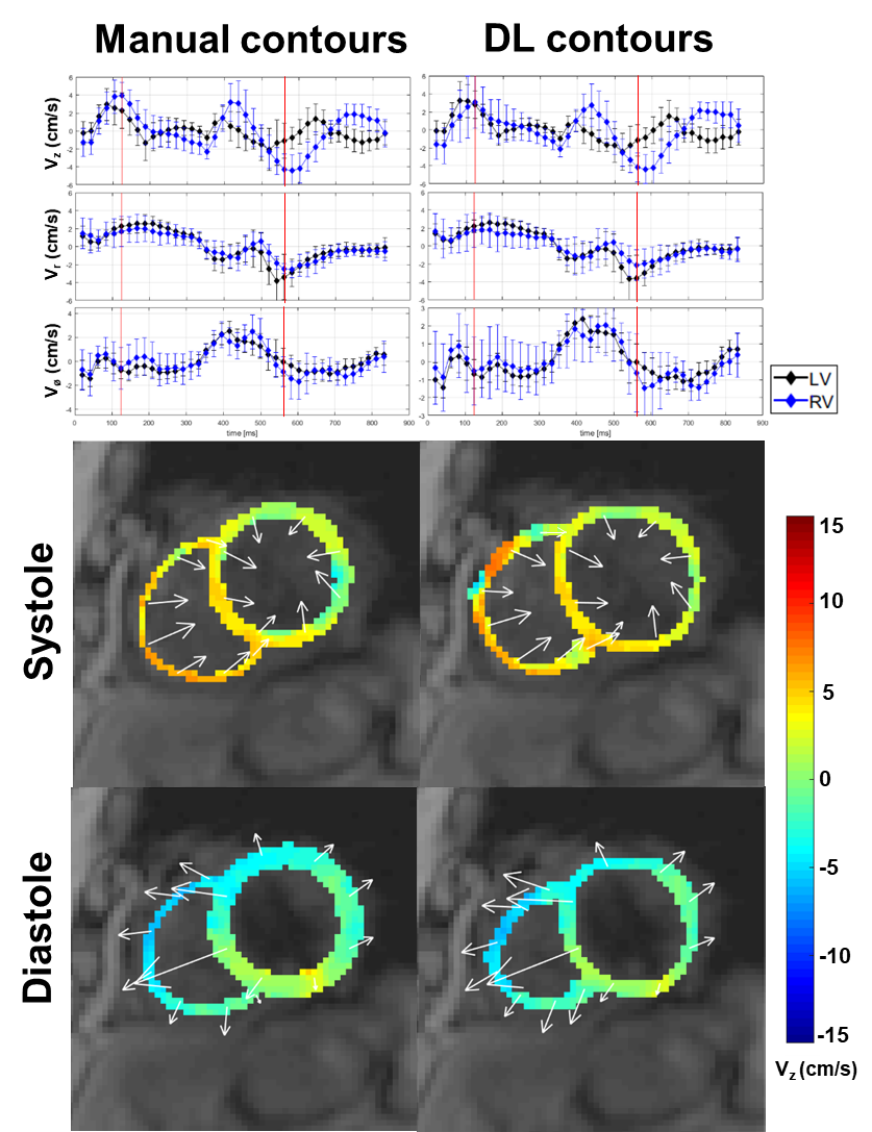
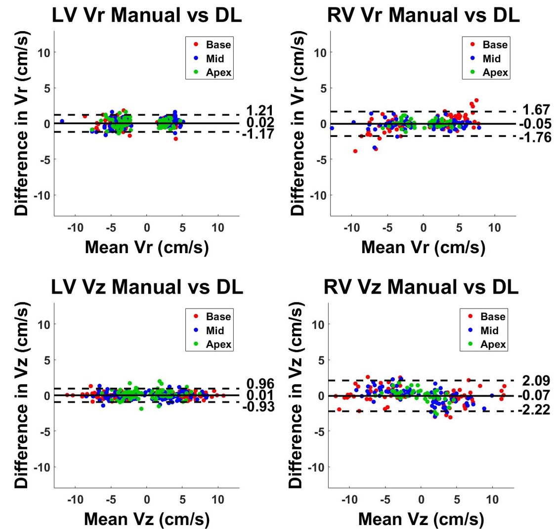
The mean segmentation time 2 hours for manual and 3.6 s for each of three U-Net architectures. Figure 3 shows results from 4 representative patients, in which 4-channel network was qualitatively slightly better than 1-channel and 2-channel network. The DICE for the LV and RV myocardium were (0.773 ± 0.105 and 0.528 ± 0.203), (0.767 ± 0.103 and 0.514 ± 0.177), (0.759 ± 0.090 and 0.567 ± 0.138) for 1-channel, 2-channel and 4-channel networks, respectively, were not significantly different (P>0.05) among all three networks. Despite the non-significant difference in DICE, we elected to use the 4-channel network because it consistently produced continuous connections in contours than other networks. Figure 4 shows representative TPM data and the corresponding velocity time curves of a patient, illustrating good agreement between manual and U-Net analyses. Figure 5 shows scatter plots resulting from the Bland-Altman analysis. The mean differences in peak radial and longitudinal velocities in LV were 0.02 cm/s (0.54% of mean of absolute values) and 0.01 cm/s (0.36% of mean of absolute values), and the limits of agreement (LOA) were 1.19 cm/s (33.3% of mean of absolute values) and 0.94 cm/s (23.3% of mean of absolute values). The mean difference in peak radial and longitudinal velocities in RV were -0.05 cm/s (-1.2 % of mean of absolute values) and -0.07 cm/s (-1.5% of mean of absolute values), and the LOA were 1.7 cm/s (43.7% of mean of absolute values) and 2.2 cm/s (48.7% of mean of absolute values).

Discussions

Our proposed 4-channel 3D residual U-Net showed the potential of automatic segmentation of the LV and RV for TPM images. While LV DICE scores for all three different networks were close to each other, 4-channel network had higher RV DICE scores and more continuous contours than other networks. Future investigation will include more datasets for training and testing, as well as explore the best network settings for different data structure.

Acknowledgements

This work was supported in part by the following grants: National Institutes of Health (R01HL116895, R01HL138578, R21EB024315, R21AG055954) and American Heart Association (19IPLOI34760317)