3515
Automated segmentation of midbrain structures using convolutional neural network1Shanghai Key Laboratory of Magnetic Resonance, School of Physics and Electronic Science, East China Normal University, Shanghai, China, 2MR Collaboration NE Asia, Siemens Healthcare, Shanghai, China, Shanghai, China, 3Department of Radiology, Weill Medical College of Cornell University, New York, NY, United States
Synopsis
Accurate
and automated segmentation of substantia nigra (SN), the subthalamic nucleus
(STN), and the red nucleus (RN) in quantitative susceptibility mapping (QSM)
images has great significance in many neuroimaging studies. In the present
study, we present a novel segmentation method by using convolution neural
networks (CNN) to produce automated segmentations of the SN, STN, and RN. The
model was validated on manual segmentations from 21 healthy subjects. Average
Dice scores were 0.82±0.02 for the SN, 0.70±0.07
for the STN and 0.85±0.04 for the RN.
Background and Purpose
The substantia nigra (SN), subthalamic nucleus (STN), and red nucleus (RN) are deep gray nuclei of great importance in studying Parkinson’s disease and movement disorder1-3. Segmentation of these structures in magnetic resonance imaging (MRI) is required and typically performed by tedious manual segmentation in quantitative assessments. Automatic segmentation of these midbrain structures is much desired but is challenging due to their fine structures and positions. The high iron contents of these structures result in high contrasts on quantitative susceptibility mapping (QSM) images4, 5, which makes it possible to automatedly segment midbrain structures using a QSM+T1 multi-atlas approach6, 7. However, the high-resolution T1-weighted images are required, and the robust performance is desired. Recently, segmentation algorithms that employ deep convolutional neural networks (CNN) have emerged as a promising solution in segmentation studies8-10. Therefore, we propose a CNN-based method for automated segmentation of SN, STN and RN in high resolution susceptibility maps.Materials and Methods
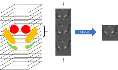
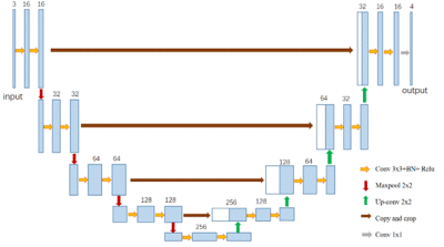
This study was approved by the local ethical committee and each participant signed an informed consent form. A total of 38 healthy subjects (28.4 ± 5.6 years old, 16 males and 22 females) underwent MRI on a clinical 3T system (MAGNETOM Prisma Fit; Siemens Healthcare, Erlangen, Germany) with a 20- channel head matrix coil. QSM was generated from a 3D spoiled multi-echo gradient-echo (GRE) sequence with the following imaging parameters: readout gradient mode = bipolar, TR = 31ms, TE1 = 4.07ms, ΔTE = 4.35ms, echoes number = 6, flip angle = 12˚, FOV = 240*288 mm2, in-plane resolution= 0.83*0.83 mm2, slice thickness = 0.8 mm, number of slices = 192. To observe the midbrain structures with minimal partial volume effects, an oblique-axial slab paralleling to the AC-PA line was chosen. QSM maps were reconstructed using the Morphology Enabled Dipole Inversion with automatic uniform cerebrospinal fluid zero reference (MEDI+0) algorithm11. The bilateral head of the SN, STN and RN were drawn manually on all QSM datasets by an experienced investigator. These steps were executed using ITK-SNAP (http://www.itk-snap.org).The datasets were split into three cohorts: 15 cases for training cohort, 2 cases for validation cohort, and 21 cases for testing cohort. Limited by the number of the cases, a slice-based CNN model was built for segmentation. The midbrain structures were located according to the brain atlas. Blocks of 64x64 size were extracted in the coronal slices. All slices including three nuclei and their adjacent slices were selected as the data set. To utilize the shape information, 3 contiguous slices were combined as the input of one sample, and the segmentation of the middle slice was labeled as the output (Figure 1)12. All slices were normalized by subtracting the mean value and dividing the standard deviation. 384 slices of training cohort and 111 slices of validation cohort were used to train the CNN model. The CNN model based on the U-Net was designed as shown in Figure 213. 3 slices were stacked in the channel direction and the segmentation result was encoded as one-hot format (Background, RN, SN, STN). To increase the robustness of the model, the augmentation involved randomly shifting, zooming, rotating, and shearing for each sample. Cross-entropy was selected as the loss function. Adam with an initial step 0.0001 was used as the optimizer14. All above were implemented using TensorFlow 1.10. We trained the model with a batch size of 20 on one NVIDIA X Titan graphics card for an hour. To evaluate the trained model, we segmented each slice of the testing cohort and then combined the segmentation into the whole brain, and we estimated the Dice score for each case.
Results
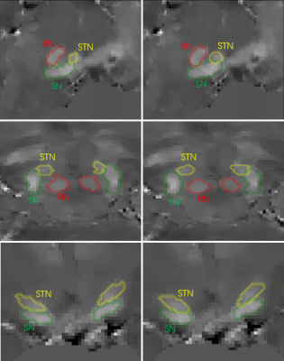
Fig. 3 shows a comparison of the manual and automated segmentations for one example case, which had the Dice scores of 0.82 for SN, 0.73 for STN and 0.87 for RN compared to the manual segmentation. The segmentation labels were overlaid on the QSM maps. The proposed CNN method accurately and consistently segmented the SN, STN and RN on high resolution susceptibility maps: Average Dice scores comparing the manual and automated segmentations were 0.82±0.02 for SN, 0.70±0.07 for STN and 0.85±0.04 for RN.Discussion and conclusions
Our preliminary data demonstrate that the CNN model has the capability to automatically segment the RN, SN and STN. This automated segmentation will eliminate the tedious manual labor in the quantitative data analysis of large Parkinson disease studies. The accuracy of the segmentation could be improved in the following aspects: 1) The performance of the CNN model may be improved using more training cases, and/or more cases synthesized by generative adversarial networks (GAN)15; 2) 3D model may be used to generate more sensitive shape and spatial information of the midbrain structures; 3) The prior experience may be combined into the model training, such as transfer learning and deformable statistics16, 17.Acknowledgements
References
1. Lewis MM, Du G, Kidacki M, et al. Higher iron in the red nucleus marks Parkinson's dyskinesia. Neurobiol Aging 2013;34:1497-1503.
2. Castrioto A, Lhommee E, Moro E, Krack P. Mood and behavioural effects of subthalamic stimulation in Parkinson's disease. Lancet Neurol 2014;13:287-305.
3. Mettler FA. Substantia Nigra and Parkinsonism. Arch Neurol 1964;11:529-542.
4. Wang Y, Spincemaille P, Liu Z, et al. Clinical quantitative susceptibility mapping (QSM): Biometal imaging and its emerging roles in patient care. J Magn Reson Imaging 2017;46:951-971.
5. Liu T, Eskreis-Winkler S, Schweitzer AD, et al. Improved subthalamic nucleus depiction with quantitative susceptibility mapping. Radiology 2013;269:216-223.
6. Garzon B, Sitnikov R, Backman L, Kalpouzos G. Automated segmentation of midbrain structures with high iron content. Neuroimage 2018;170:199-209.
7. Li X, Chen L, Kutten K, et al. Multi-atlas tool for automated segmentation of brain gray matter nuclei and quantification of their magnetic susceptibility. Neuroimage 2019;191:337-349.
8. Li X, Chen H, Qi X, Dou Q, Fu CW, Heng PA. H-DenseUNet: Hybrid Densely Connected UNet for Liver and Tumor Segmentation From CT Volumes. IEEE Trans Med Imaging 2018;37:2663-2674.
9. Liu F, Zhou Z, Jang H, Samsonov A, Zhao G, Kijowski R. Deep convolutional neural network and 3D deformable approach for tissue segmentation in musculoskeletal magnetic resonance imaging. Magn Reson Med 2018;79:2379-2391.
10.Chen H, Zhang Y, Kalra MK, et al. Low-Dose CT With a Residual Encoder-Decoder Convolutional Neural Network. IEEE Trans Med Imaging 2017;36:2524-2535.
11.Liu Z, Spincemaille P, Yao Y, Zhang Y, Wang Y. MEDI+0: Morphology enabled dipole inversion with automatic uniform cerebrospinal fluid zero reference for quantitative susceptibility mapping. Magnetic Resonance in Medicine 2018;79:2795-2803.
12.De Fauw J, Ledsam JR, Romera-Paredes B, et al. Clinically applicable deep learning for diagnosis and referral in retinal disease. Nat Med 2018;24:1342-1350.
13.Ronneberger O, Fischer P, Brox T. U-Net: Convolutional Networks for Biomedical Image Segmentation.
14.Kingma DP, Ba J. Adam: A Method for Stochastic Optimization. arXiv:14126980 2014.
15.Goodfellow IJ, Pouget-Abadie J, Mirza M, et al. Generative Adversarial Networks. arXiv:14062661 2014.
16.Dong S, Luo G, Wang K, Cao S, Li Q, Zhang H. A Combined Fully Convolutional Networks and Deformable Model for Automatic Left Ventricle Segmentation Based on 3D Echocardiography. Biomed Res Int 2018;2018:5682365.
17.Tan C , Sun F , Kong T , et al. A Survey on Deep Transfer Learning. arXiv:18080741 2018.


