3501
VIOLIN: improVIng mOdel-based deep learning reconstruction by reLaxing varIable combiNations1Shenzhen Institutes of Advanced Technology, Chinese Academy of Sciences, Shenzhen, China, 2Nanchang University, Nanchang, China, 3University at Buffalo, The State University of New York, Buffalo, Buffalo, NY, United States
Synopsis
Most of the unrolling-based deep learning fast MR imaging methods learn the parameters and regularization functions with the network architecture structured by the corresponding optimization algorithm. In this work, we introduce an effective strategy, VIOLIN and use the primal dual hybrid gradient (PDHG) algorithm as an example to demonstrate improved performance of the unrolled networks via breaking the variable combinations in the algorithm. Experiments on in vivo MR data demonstrate that the proposed strategy achieves superior reconstructions from highly undersampled k-space data.
Introduction
Deep learning (DL) has been incorporated into MR imaging for improving the quality of reconstructed image from highly undersampled k-space data1-6. Specifically, model-driven methods have shown great promise by unrolling the optimization algorithms to deep networks, allowing the uncertainties in the model to be learned through network training3-5. Most of these unrolling-based methods learn the parameters and regularization functions with the network architecture structured by the corresponding optimization algorithm. However, their performance can be improved with further utilizing the strong learning ability of deep networks. In this work, we use the primal dual hybrid gradient (PDHG) algorithm7 as an example to demonstrate improved performance of the unrolled networks via relaxing the variable combination in the algorithm. Experimental results show that the proposed strategy can achieve superior results from highly undersampled k-space data.Theory
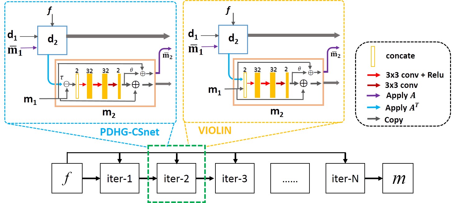
The unconstrained image reconstruction model can be formulated as$$\min_{m}\frac{1}{2} ‖Am-f‖_2^2+λG(m) (1)$$where $$$m$$$ is the image to be reconstructed, $$$A$$$ is the encoding matrix, $$$f$$$ denotes the acquired k-space data, and $$$G(m)$$$ denotes the regularization function. With PDHG algorithm, the solution of problem (1) is$$\begin{cases}d_{n+1}=\frac{d_n+σ(A\overline{m}_n-f)}{1+σ} \\m_{n+1}=prox_τ [G](m_n-τA^* d_{n+1}) \\\overline{m}_{n+1 }=m_{n+1}+θ(m_{n+1}-m_n)\end{cases} (2)$$where $$$σ$$$, $$$τ$$$ and $$$θ$$$ are the algorithm parameters, and $$$prox$$$ denotes the proximal operator, which can be obtained by the following minimization:$$prox_τ [G](x)=\arg min_{z}\left\{G(z)+\frac{‖z-x‖_2^2}{2τ}\right\} (3)$$ A learnable operator, which is the convolutional neural network (CNN), is used to replace the proximal operator in (2), thus, the unrolled network, called PDHG-CSnet8, can be formed as$$\begin{cases}d_{n+1}=\frac{d_n+σ(A\overline{m}_n-f)}{1+σ} \\m_{n+1}=Λ(m_n-τA^* d_{n+1}) \\\overline{m}_{n+1 }=m_{n+1}+θ(m_{n+1}-m_n)\end{cases} (4)$$The parameters $$$σ$$$, $$$τ$$$ and $$$θ$$$and the operator $$$Λ$$$ are all learned by the network.Noticed that the update of the CNN input is explicitly enforced as $$$m_n-τA^* d_{n+1}$$$. To better utilize the learning capability of deep networks and further improve the reconstruction quality, we break the updating structure such that the combinations of the variables are freely learned by the network. Then, the new network can be formulated as $$\begin{cases}d_{n+1}=\frac{d_n+σ(A\overline{m}_n-f)}{1+σ} \\m_{n+1}=Λ(m_n,A^* d_{n+1}) \\\overline{m}_{n+1 }=m_{n+1}+θ(m_{n+1}-m_n)\end{cases} (5)$$
Methods
The structure of the proposed network is shown in Fig 1. The convolutions are all 3x3 pixel size, and implemented in TensorFlow using two separate channels representing the real and imaginary parts of MR data.We trained the networks using in-vivo MR datasets. Overall 2100 fully sampled multi-contrast data from 10 subjects with a 3T scanner (MAGNETOM Trio, SIEMENS AG, Erlangen, Germany) were collected and informed consent was obtained from the imaging object in compliance with the IRB policy. The fully sampled data was acquired by a 12-channel head coil with matrix size of 256×256 and adaptively combined to single-channel data and then retrospectively undersampled using Poisson disk sampling mask. 1600 fully sampled data were used to train the networks. We tested the proposed methods on 398 human brain 2D slices, which were acquired from SIEMENS 3T scanner with 32-channel head coil and 3D T1-weighted SPACE sequence, TE/TR=8.4/1000ms, FOV=25.6×25.6×25.6cm3. The data was fully acquired and then manually combined to single-channel and down-sampled for reconstruction. The networks have also been tested on the fully sampled data from another commercial 3T scanner (United Imaging Healthcare, Shanghai, China).
Results
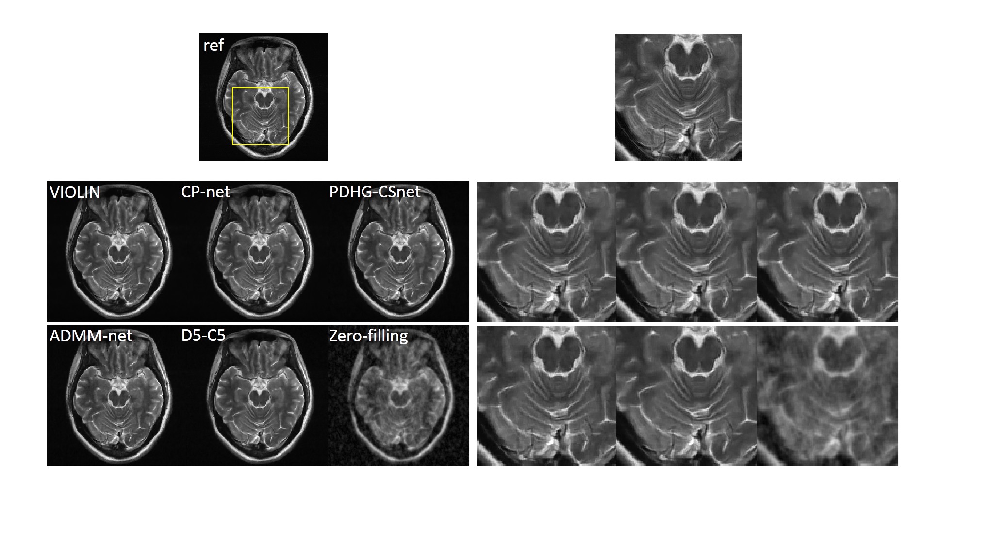
As the variable combinations in the algorithm (4) are relaxed, the quality of the reconstruction gets better, which is shown in Fig. 2.We also compared the proposed network with other reconstruction methods: 1) CP-net8, an unrolling version of PDHG algorithm with the learned data consistency; 2) generic-ADMM-CSnet (ADMM-net)3, an unrolling-based deep learning method learning the regularization function; 3) D5-C52, a deep learning method with data consistency; 4) zero-filling, the inverse Fourier transform of undersampled k-space data. The visual comparisons are shown in Fig. 3. The zoom-in images of the enclosed part and the corresponding quantitative metrics are also provided.
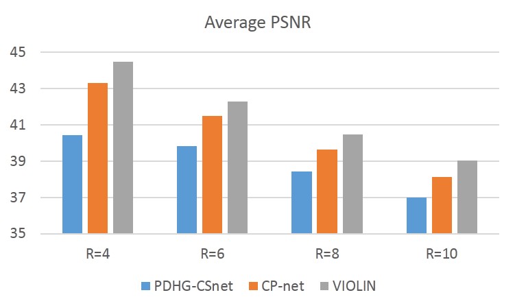
The average performance of VIOLIN on the 398 brain data with different acceleration factors can be seen in Fig 4. The quality of reconstruction deteriorates with larger acceleration factors for each network. Whereas for the fixed acceleration factor, the performance improvement induced by relaxing can be observed. It is worth noting that the relaxation of variable combination plays a more important role in improving reconstruction quality than that of data consistency, as compared with CP-net.
Conclusion
In this work, we proposed an effective way to improve the reconstruction quality of unrolling-based deep networks. The effectiveness of the proposed strategy was validated on in vivo MR data. The extension to multi-channel MR acquisitions and other algorithms will be explored in the future.Acknowledgements
This work was supported in part by the National Natural Science Foundation of China (U1805261), National Key R&D Program of China (2017YFC0108802) and he Strategic Priority Research Program of Chinese Academy of Sciences (XDB25000000).References
1. Wang S, Su Z, Ying L, et al. Accelerating magnetic resonance imaging via deep learning. ISBI 514-517 (2016)
2. Schlemper J, Caballero J, Hajnal J V, et al. A Deep Cascade of Convolutional Neural Networks for Dynamic MR Image Reconstruction. IEEE TMI 2018; 37(2): 491-503.
3. Yang Y, Sun J, Li H, Xu Z, ADMM-CSNet: A Deep Learning Approach for Image Compressive Sensing. IEEE Trans Pattern Anal Mach Intell, 2018.
4. Hammernik K, Klatzer T, Kobler E, et al. Learning a Variational Network for Reconstruction of Accelerated MRI Data. Magn Reson Med 2018, 79(6): 3055-3071.
5. Zhang J, Ghanem B. ISTA-Net: Interpretable Optimization-Inspired Deep Network for Image Compressive Sensing. CVPR 2018, 1828-1837.
6. Zhu B, Liu J Z, Cauley S F, et al. Image reconstruction by domain-transform manifold learning. Nature 2018; 555(7697): 487-492.
7. Chambolle A, Pock T. A First-Order Primal-Dual Algorithm for Convex Problems with Applications to Imaging. J. Math. Imag. Vis. 2011; 40:120-145.
8. Cheng J, Wang H, Ying L, Liang D. Model Learning: Primal Dual Networks for Fast MR Imaging. MICCAI 2019
Figures