Introduction

Analysing T₂ relaxation times as a continuous distribution is an intrinsically ill-posed problem. The traditional inverse Laplace transform (ILT) employs a non-negative constraint and a user defined regularization parameter for spectrum smoothness [1]. ANNs have been applied to T₂ distribution analysis for myelin fraction evaluation [2], mainly for the advantage of fast computation speed, with ANN trained based on the ILT results. Therefore, the performance should not exceed that of the ILT. In this work, ANNs were trained with signals simulated with continuous T₂ spectra, and higher accuracy was achieved, compared to ILT.

Methods

Network Architecture
Keras [3] and NumPy [4] were employed to create the networks, with an array of the decay signal values as input and spectrum amplitude as output. The network hyperparameters were determined by an evolutionary algorithm [5] (activation function: selu [6], optimizer: Adam [7], batch size: 256, epochs: 500, 6 layers resembling an hourglass shape narrower in the centre with the number of nodes ranging from 2500 to 1000). For each SNR, 4 ANNs were trained with the number of nodes varying randomly by approximately 25%. The results were averaged as the final output to ensure no singularities occurred. Loss function was the sum of mean squared errors of the spectrum and the decay curve compared to the noiseless decay and a factor to punish negative values.
Training Dataset
400 000 multiple spin echo decay signals, with equally spaced (ES) data points, were simulated for each SNR (2000 and 80). T₂ values were in the unit of ES, in the dynamic range of ES to ES×512 (number of echoes). The spectrum amplitude values were normalized. Rician noise [8] was added to the scaled decay signals, by including zero-mean Gaussian noises in the real and imaginary channels, separately.
Three Gaussian functions were generated with random widths, positions and relative heights on a logarithmic scale. The distribution spectrum amplitude was the sum of the three Gaussian functions. The positions of the three peaks might overlap or partially overlap, so that spectra with one or two peaks were included in the training data set.
Network evaluation
Simulations and experimental data, with one-peak and two-peak T₂ distribution spectra of various peak widths, peak positions and peak area ratios were tested with the ANNs. The results were compared with ILT, where applicable.

Results and Discussion

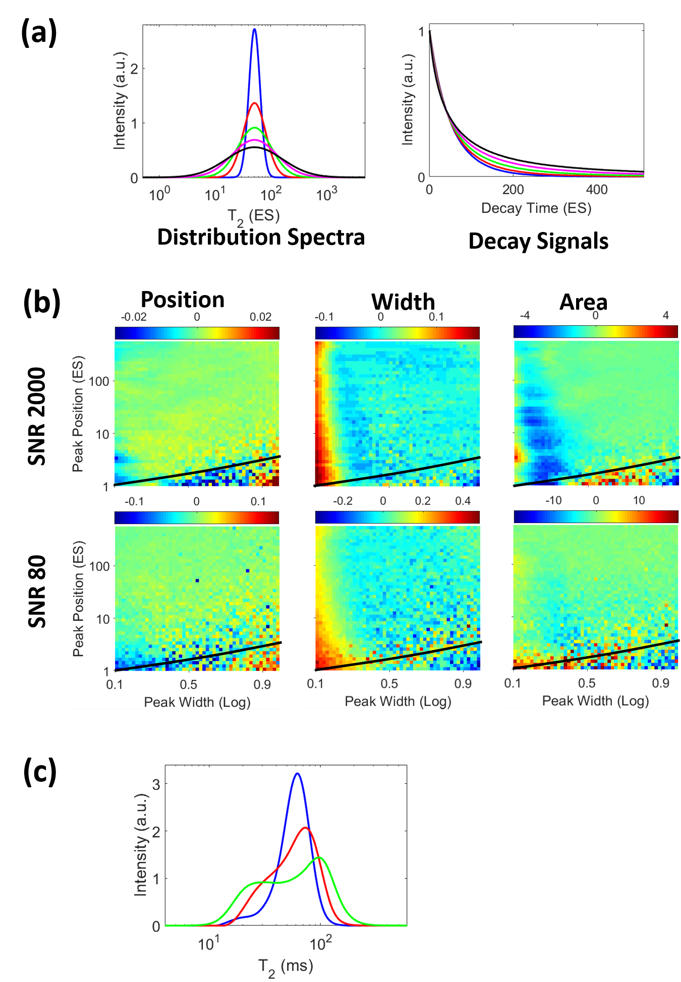
Peak width detection
The peak width information is generally not available in the ILT results, since it is defined by the regularization parameter. Simulations of single peak spectra with various peak widths and corresponding decay signals, shown in Fig. 1a, suggested that the peak width information should be available within the SNR limit. Single peak spectra, with varying mean T₂ values (peak position) and peak width, were simulated with SNR 2000 and SNR 80. The error maps of the ANN results are shown in Fig. 1b. ANN was able to accurately determine the peak position, area, and width except for very narrow peaks, where the dynamic range of coefficients was large. This could be mitigated by training a separate ANN with only narrow peaks. Fig. 1c shows phantom measurement results that the spectra widths were accurately determined.
Two-peak spectra evaluations
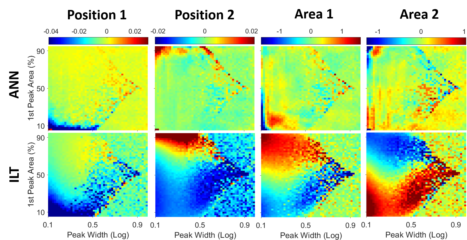
The accuracy of the T₂ distribution analysis depends on many factors, such as the peak positions, peak widths, and relative areas under the peak (quantities of each component). Spectra with fixed T₂ positions, at 20 ES and 200 ES, were simulated with varying peak width and area ratio. Error maps in the log mean positions and the peak areas were compared with the ILT results, as shown in Fig. 2. The ANN errors were very low, while large systematic errors were observed in ILT.
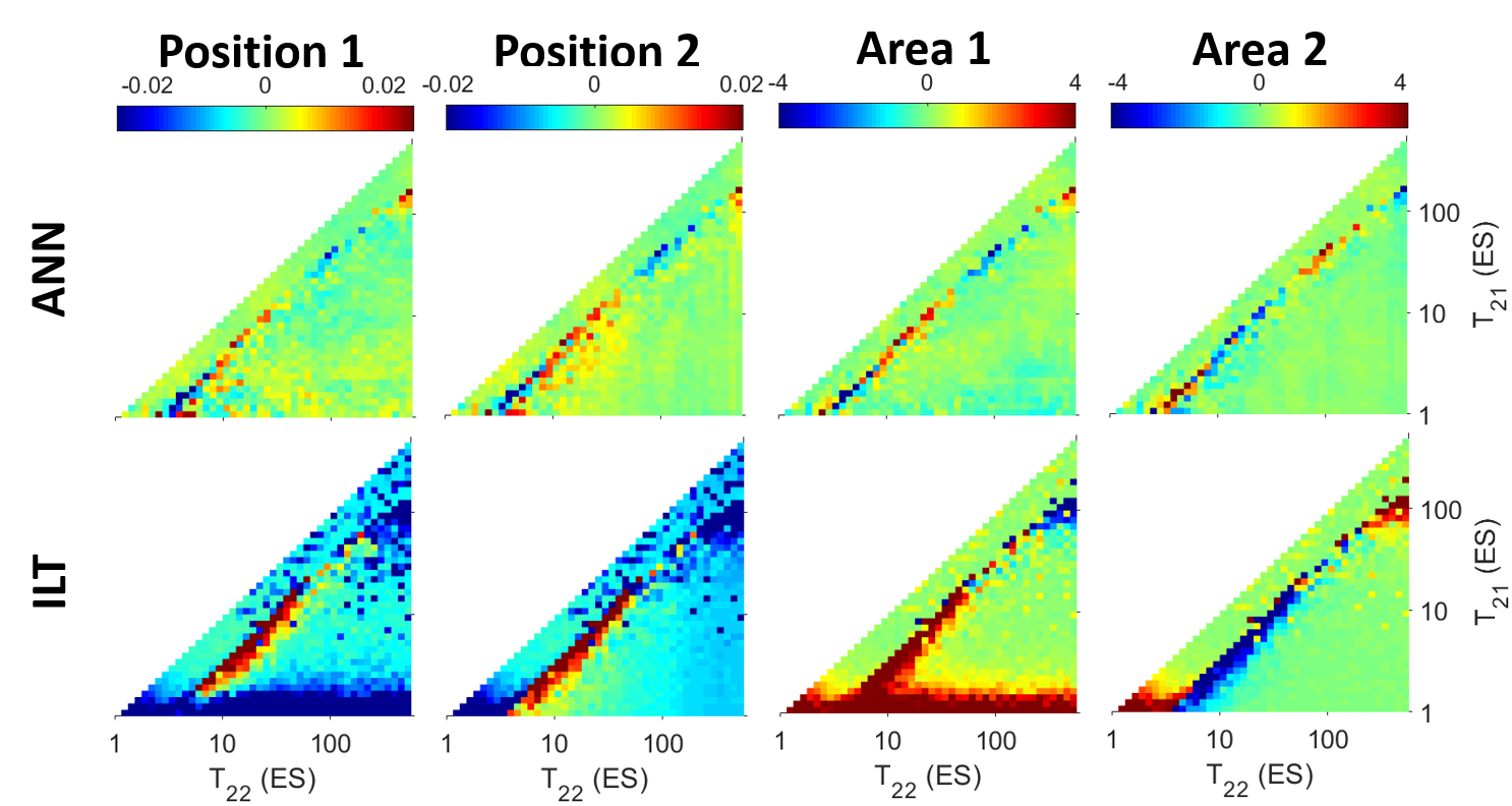
Spectra with varying peak positions were simulated, with fixed area ratio (50:50) and peak width (0.3). The error maps are shown in Fig. 3. In the diagonal sections to the left of the distinct boundaries, only one peak was detected. This highlighted the resolution limit, at a factor of approximately 3 for ILT and slightly smaller for ANN, which agreed with the literature [9]. Large errors were observed in ILT especially in the position and area of the first peak with very small short T₂ values, as well as when the separation of the two peaks was close to the resolution limit.
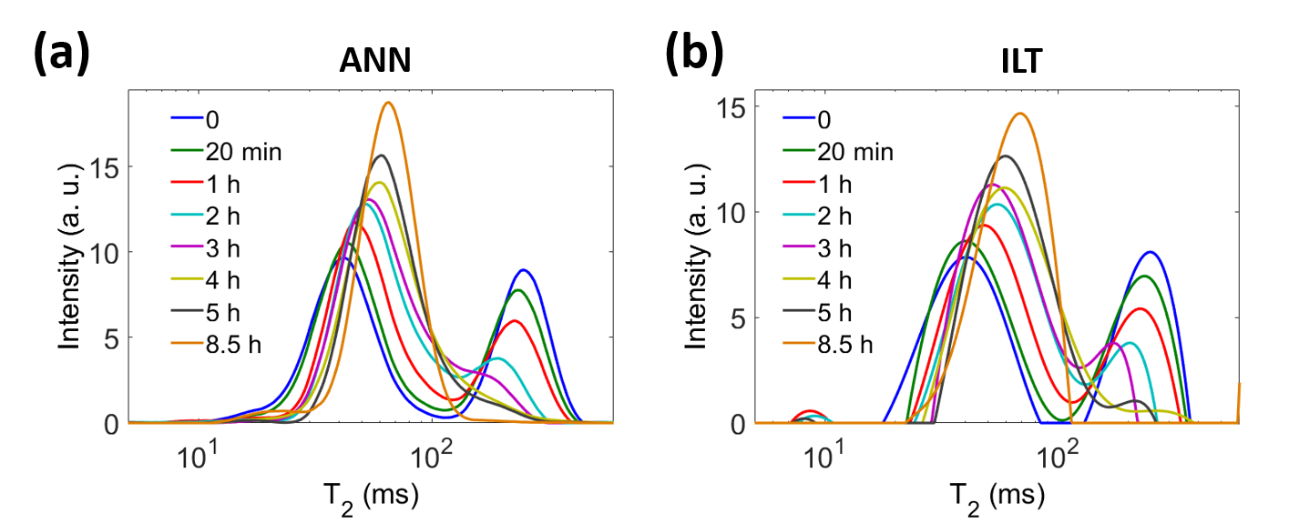
CPMG measurements were performed on a phantom consisting of an Agar gel (T₂ ≈ 250 ms) in contact with doped CuSO₄ solution (T₂ ≈ 40 ms), through a duration of 8.5 hours. The dynamic spectra are shown in Figure 4. The quantities and values of both components changed with time, as the CuSO₄ migrated into the gel. The two peaks merged into one after 4 hours, and the peak width became narrower after as the relaxation rates within the sample became more homogeneous. ANN generated dynamic T₂ spectra with a smoother transition than ILT.

Conclusion

We demonstrated the effectiveness of ANN for analyzing continuous T₂ distribution. Spectra width, usually considered not available, can be obtained when the SNR permitted. The performance was evaluated across a large parameter space, and was superior compared to the traditional ILT method.

Acknowledgements

T.P. thanks NSERC of CANADA for a USRA and the University of Windsor Outstanding Scholars Program. D.X. thanks NSERC of Canada for a Discovery grant. We thank Dr. Martin Hürlimann for providing the ILT algorithm and helpful discussions.