3477
Accelerated MR-STAT Algorithm: Achieving 10-minute High-Resolution Reconstructions on a Desktop PC1Computational Imaging Group for MR Diagnostics and Therapy, Center for Image Sciences, University Medical Center Utrecht, Utrecht, Netherlands, 2Department of Radiology, Division of Imaging and Oncology, University Medical Center Utrecht, Utrecht, Netherlands
Synopsis
MR-STAT is a framework for simultaneous mapping of quantitative MR parameters from a single short scan. Since MR-STAT involves the solution of a large scale nonlinear optimization problem, the reconstruction time has always been one main concern. In the current work, we develop an accelerated MR-STAT algorithm, which achieves two order of magnitude acceleration in reconstruction times. High-resolution 2D dataset can be reconstructed within 10 minutes on a desktop PC thereby drastically facilitating the application of MR-STAT in the clinical work-flow.
Introduction
MR-STAT is a framework for obtaining multi-parametric quantitative maps from single short scan[1,2]. The parameter maps are reconstructed by iteratively solving the large scale, non-linear problem$$\hat{\alpha }=\arg\min_{\alpha }\frac{1}{2}\left\Vert d-s( \alpha )\right\Vert^{2}_{2},\ \ \ (1)$$
where $$$d$$$ is the data in time domain, $$$\alpha$$$ denotes all parameter maps, and $$$s$$$ is the volumetric signal model. Although recent improvements have been obtained[2,3], MR-STAT reconstructions still lead to long computation times because of the large scale of the problem, requiring a high performance computing cluster for application in a clinical work-flow.
In this work, we drastically accelerate MR-STAT reconstructions by following two strategies, namely: 1) computing the signal and derivatives by a fast surrogate model and 2) adopting an Alternative Direction Methods of Multipliers[4]. The new algorithm achieves a two order of magnitude acceleration in reconstructions with respect to the state-of-the-art MR-STAT. A high-resolution 2D dataset is reconstructed within 10 minutes on a desktop PC thereby greatly facilitating the application of MR-STAT in the clinical work-flow.
Theory
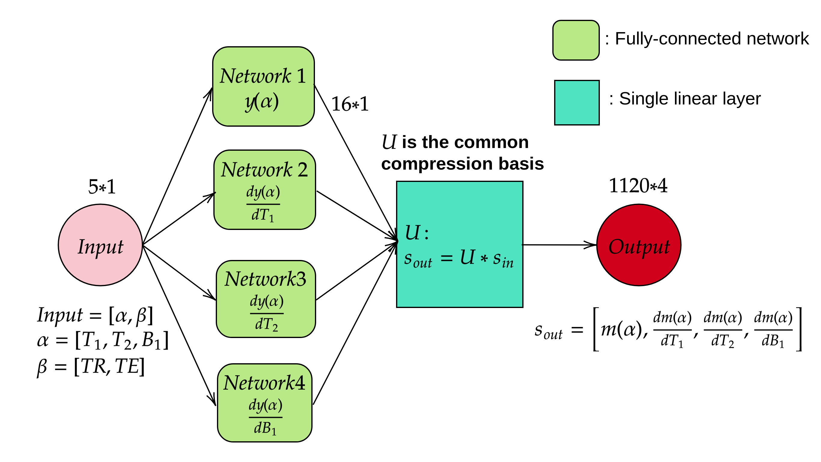
- Surrogate MR signal Model
- The ADMM approach
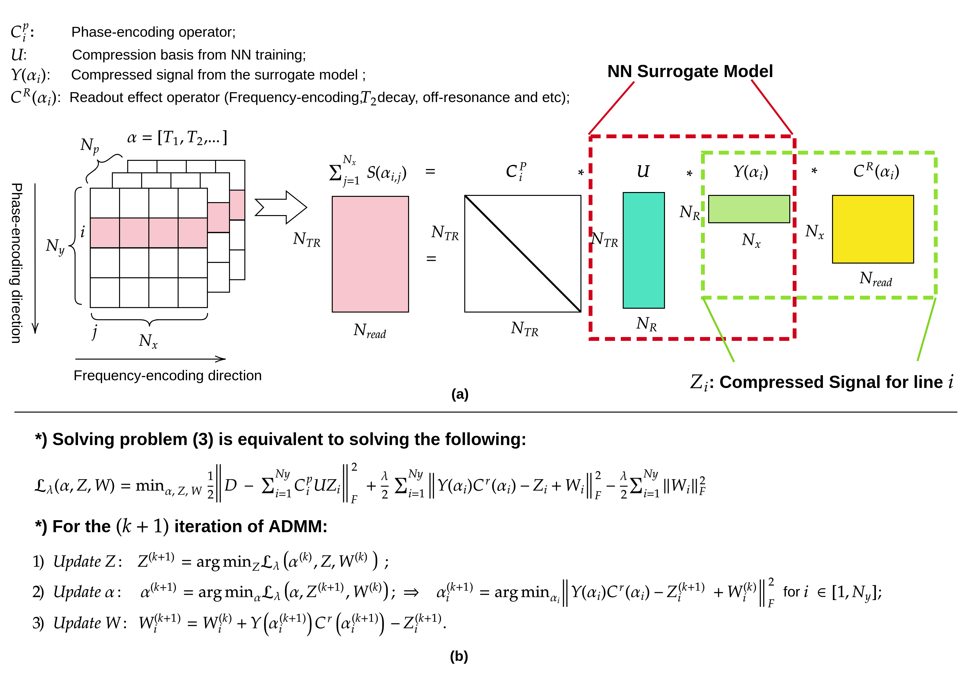
$$\hat{\alpha}=\arg\min_{\alpha}\frac{1}{2}\left\Vert D-\sum^{Ny}_{i=1}C^{p}_{i}UY(\alpha _{i})C^{r}(\alpha _{i})\right\Vert^{2}_{F}.\ \ \ (2)$$
A graphic illustration of the new problem (2) and the explanation of the operators is shown in Figure 2(a).
We reformulate problem (2) as the following constrained problem
$$\hat{\alpha}=\arg\min_{Z,\alpha}\frac{1}{2}\left\Vert D-\sum^{Ny}_{i=1}C^{p}_{i}UZ_{i}\right\Vert^{2}_{F} \text{subject to }Y(\alpha _{i})C^{r}(\alpha _{i})-Z_{i}=0\text{ for }i\in [1,N_{y}],\ \ \ (3) $$
by adding slack variable $$$Z_i$$$. The corresponding alternating update scheme[4] is shown in Figure 2(b). In this scheme, step (1) solves a linear problem and step (2) solves $$$N_x$$$ small parallelizable nonlinear problems using the compressed signal, therefore substantially reducing the computational complexity w.r.t. the original MR-STAT.
Methods
Both balanced and gradient spoiled MR-STAT sequence are used in the current work with Cartesian acquisition and slowly varying flip angle trains[2].- Surrogate model training and validation
- Accelerated MR-STAT reconstruction
For in-vivo validation, the standard and accelerated MR-STAT reconstructions are run on both gradient spoiled (scan time 9.8s, TR=8.7ms, TE= 4.6ms) and balanced (scan time 10.3s, TR=9.16ms, TE=4.58ms) acquisitions.
Results
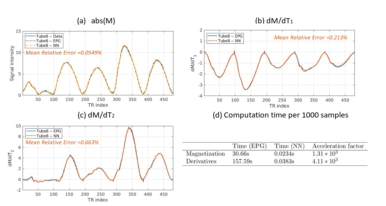
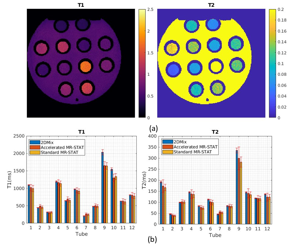
Figure 3 summarizes the validation results of the surrogate MR signal model, showing that the NN surrogate model achieves an acceleration factor of thousand with negligible errors.Figure 4 shows high agreements in $$$T_1$$$ and $$$T_2$$$ maps obtained from standard MR-STAT reconstruction, accelerated MR-STAT reconstruction and a 2DMix acquisition for the gel phantom data.
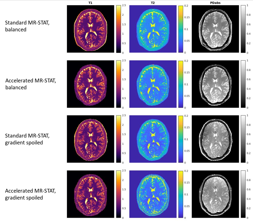
Figure 5 shows in-vivo results of one representative slice from a healthy human brain; both standard and accelerated MR-STAT algorithms obtain similar quantitative maps from both balanced and gradient spoiled acquisitions.
With the accelerated MR-STAT algorithm, one 2D slice reconstruction requires approximately 157 seconds with single-coil data, and 671 seconds with four compressed virtual coil data. Compared with the results reported previously (50 minutes single-coil reconstruction on a 64 CPU's cluster[3]), our accelerated algorithm obtains a two order of magnitude acceleration in reconstruction time.
Conclusion and Discussion
We presented a new MR-STAT reconstruction algorithm where both a Neural Network surrogate model and a variable splitting scheme are employed. Simulated, phantom and in-vivo experiments show that the new MR-STAT algorithm is two orders of magnitude faster than the conventional algorithm and can thus run in 10 minutes on a Desktop PC. Training of the NN takes about two hours in total, but the network is flexible and can be reused for sequences with different parameters (TE, TR).This new implementation paves the way to the application of MR-STAT in the clinic, since the computation time is no longer a burden for the clinical work-flow.
Acknowledgements
The first author receives CSC(Chinese Scholarship Counsel) scholarship.
References
[1] Sbrizzi, Alessandro, et al. "Fast quantitative MRI as a nonlinear tomography problem." Magnetic resonance imaging 46 (2018): 56-63.
[2] van der Heide, Oscar, et al. "High resolution in-vivo MR-STAT using a matrix-free and parallelized reconstruction algorithm." arXiv preprint arXiv:1904.13244 (2019).
[3] van der Heide, Oscar, et al. "Sparse MR-STAT: Order of magnitude acceleration in reconstruction times." in ISMRM, Montreal, Canada, p. 4538 (2019).
[4] Boyd, Stephen, et al. "Distributed optimization and statistical learning via the alternating direction method of multipliers." Foundations and Trends in Machine learning 3.1 (2011): 1-122.
[5] Weigel, Matthias. "Extended phase graphs: dephasing, RF pulses, and echoes‐pure and simple." Journal of Magnetic Resonance Imaging 41.2 (2015): 266-295.
[6] Abadi, Martín, et al. "Tensorflow: Large-scale machine learning on heterogeneous distributed systems." arXiv preprint arXiv:1603.04467 (2016).
[7] In den Kleef, J. J. E., and J. J. M. Cuppen. "RLSQ: T1, T2, and ρ calculations, combining ratios and least squares." Magnetic resonance in medicine 5.6 (1987): 513-524.
Figures