3474
Sparse sampling reconstruction and noise removal of 0.55T brain MRI using a learned variational network
Patricia M. Johnson1, Zhang Le2, David Grodzki3, and Florian Knoll1
1Center for Biomedical Imaging, New York University, New york, NY, United States, 2Siemens Shenzhen Magnetic Resonance Ltd., Shenzhen, China, 3Siemens Healthcare GmbH, Erlangen, Germany
1Center for Biomedical Imaging, New York University, New york, NY, United States, 2Siemens Shenzhen Magnetic Resonance Ltd., Shenzhen, China, 3Siemens Healthcare GmbH, Erlangen, Germany
Synopsis
Most clinical MRI scanners operate at high magnetic field, however low-field MRI offers many advantages and promises to improve the value of MRI. The main drawback is low SNR; several signal averages are often required, which may result in prohibitively long scans. We can look to deep learning (DL) to facilitate accelerated low-field imaging through both denoising and sparse sampling. In this work, we use a variational network for both denoising and under-sampled reconstruction of brain images acquired on a 0.55T prototype system, demonstrating that low-field MRI paired with DL can produce high-quality images in very short scan times.
Introduction
Most clinical MRI scanners operate at high magnetic fields, with the most common field strengths being 1.5T and 3T. Traditionally, low-field scanners have been less attractive, because the reduced signal-to-noise ratio (SNR) may result in degraded image quality. However, systems with lower magnetic fields do offer significant advantages. The lower cost of installation and maintenance could improve access to MRI globally. Additionally, low-field magnets have smaller fringe fields making placement of the system far more versatile, potentially enabling point-of-care imaging [1]. In low-field systems, there is also a reduction of SAR, RF heating, and susceptibility artifacts.The development of low-field systems promises to expand the value and utility of MRI and improve access. However, several signal averages are often required in order to achieve diagnostic SNR, which may result in prohibitively long scan times. Many of the applications for which low-field imaging is well suited demand fast imaging, for example, MR-guided surgical interventions [2], and MR imaging in an acute setting [3]. Two potential approaches for acquiring high-quality low-field images in a clinically feasible scan time are denoising and sparse sampling reconstruction.
Low-field and accelerated imaging have significant potential for improving global access and value of MRI. We can look to deep learning (DL) to facilitate accelerated low-field imaging through both denoising and sparse sampling. Denoising using convolutional neural networks (CNNs) has been demonstrated previously for both X-ray [4] and CT imaging [5]. Additionally, DL based reconstruction of under-sampled MR images is an active area of research [6-8]. One promising method is the variational network (VN). In this work, we adopt a VN approach for both denoising and under-sampled reconstruction of brain images acquired on a 0.55T prototype system, demonstrating that low field MRI paired with DL can produce high-quality images in very short scan times.
Methods
System and data26 subjects were scanned using a prototype MAGNETOM Aera (Siemens Healthcare, Erlangen, Germany), modified to operate at 0.55T, and a 12-channel head coil. The acquisition is a T2-weighted, turbo spin echo sequence with parameters as follows: TR$$$\thinspace$$$=$$$\thinspace$$$5.75$$$\thinspace$$$s, turbo factor$$$\thinspace$$$=$$$\thinspace$$$15, slice thickness$$$\thinspace$$$=$$$\thinspace$$$5$$$\thinspace$$$mm, FOV = 23 x 20 $$$\thinspace$$$cm, in-plane resolution = 0.45 x 0.45$$$\thinspace$$$mm, averages = 6, scan time =$$$\thinspace$$$14.5$$$\thinspace$$$mins
Variational network (VN)
The VN originally described in Hammernik et al. [7] is a DL-based reconstruction technique. Using the zero-filled reconstruction as the starting point, the VN solves the image reconstruction problem by enforcing k-space data consistency, application of the measured coil sensitivities, and using a CNN to learn the regularizer. In this work, we modified the original VN by replacing the regularizer with a Unet [9]. This results in a higher model capacity regularizer (1.2 million parameters) with a larger receptive field.
Training
To train the VN for denoising we use training pairs where the input is raw multi-channel k-space data from a single (noisy) acquisition, and the target is an average of multiple acquisitions. With the network enforcing data consistency in every layer, it is performing a true denoising reconstruction. A total of 5 networks were trained where the target image data were two-six signal averages. With these experiments we can evaluate the effect of target SNR on the denoising performance of the network.
To train the VN for sparse sampling reconstruction we use training pairs where the input is a 2x or 3x retrospectively under-sampled single acquisition and the target is an average of all 6 fully-sampled acquisitions. For the input data, we used parallel imaging style, regular spaced under-sampling with 24 calibration lines.
For all experiments, the training/validation/test split was 16/5/5/ volumes. The VN was trained with the Adam optimizer, a learning rate of 1x10⁻³ and a batch size of 1. The number of epochs were 15 and 25 for the denoising and sparse-sampling experiments respectively.
Results
Denoising reconstructionTo quantitatively evaluate the reconstructed image quality, we used structural similarity index (SSIM). A plot of SSIM vs. the number of target signal averages is shown in figure 1. The mean SSIM – calculated over all slices in the test set – increases with an increasing number of target averages. The improvement plateaus at about 4 averages. Example images for all five trained networks are shown in figure 2.
Sparse sampling reconstruction
Zero-filled reconstruction of 2x and 3x under-sampled images resulted in a mean SSIM of 0.76 ±0.05 and 0.73 ±0.05 respectively. The reconstructed images have aliasing and low SNR as expected. VN reconstruction of 2x and 3x under-sampled images resulted in a mean SSIM of 0.89 ±0.03 and 0.87 ±0.03. The VN reconstruction successfully removes aliasing and noise from the images. Example images are shown in figure 3.
Discussion/Conclusions
A VN successfully removed noise during image reconstruction of 0.55T MRI data. Our results show that image quality improves when more signal averages are used for the target during training; however, there is minimal improvement beyond 4 averages. Our results show that by combining denoising and undersampled reconstruction, the original scan time of 14.5$$$\thinspace$$$mins could be reduced to 54$$$\thinspace$$$s – a 16-fold acceleration. Approaches that combine DL-based image reconstruction with low-field acquisitions may be able achieve image quality comparable to high-field imaging, with the significant benefit of improved access and utility.Acknowledgements
We acknowledge grant support from the National Institutes of Health, grants NIH R01 EB024532 and NIH P41 EB017183. We also acknowledge the support of the Natural Sciences and Engineering Research Council of Canada (NSERC); P. Johnson is the recipient of an NSERC Postdoctoral fellowship award.References
- Panther, A. et al., A Dedicated Head-Only MRI Scanner for Point-of-Care Imaging. in ISMRM. 2019. Montreal.
- Campbell-Washburn, A.E., et al., Opportunities in Interventional and Diagnostic Imaging by Using High-Performance Low-Field-Strength MRI. Radiology, 2019. 293(2): p. 384-393.
- Stainsby, J.A. et al., High-Performance Diffusion Imaging on a 0.5T System. in ISMRM. 2019.
- Green, M., et al., Neural Denoising of Ultra-low Dose Mammography, Machine Learning for Medical Image Reconstruction. MLMIR 2019. Lecture Notes in Computer Science, vol 11905.
- Kang, E., J. Min, and J.C. Ye, A deep convolutional neural network using directional wavelets for low-dose X-ray CT reconstruction. Med Phys, 2017. 44(10): p. e360-e375.
- Aggarwal, H.K., M.P. Mani, and M. Jacob, MoDL: Model-Based Deep Learning Architecture for Inverse Problems. IEEE Trans Med Imaging, 2019. 38(2): p. 394-405.
- Hammernik, K., et al., Learning a Variational Network for Reconstruction of Accelerated MRI Data. Magn Reson Med, 2018. 79(6): p. 3055-71.
- Zhu, B., et al., Image reconstruction by domain-transform manifold learning. Nature, 2018. 555(7697): p. 487-492.
- Ronneberger, O., P. Fischer, and T. Brox, U-Net: Convolutional Networks for Biomedical Image Segmentation. Medical Image Computing and Computer-Assisted Intervention – MICCAI 2015. MICCAI 2015. Lecture Notes in Computer Science. 9351.
Figures

Figure 1. Plot of SSIM vs the number of signal averages
for the target image. The values shown are mean and standard deviation. SSIM improves when the SNR of the target image increases,
until a plateau is reached at about 4 signal averages.
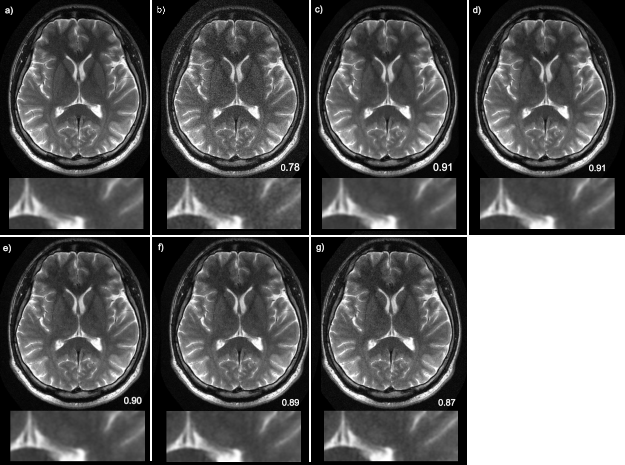
Figure 2. Example
result demonstrating denoising of a T2-weighted brain image. The target image, which is an average of 6
acquisitions, is shown in (a). The input image, which is a single acquisition, is
shown in (b). The variational network reconstructions for the 6-avg, 5-avg,
4-avg, 3-avg and 2-avg trained networks are shown in (c)-(g).
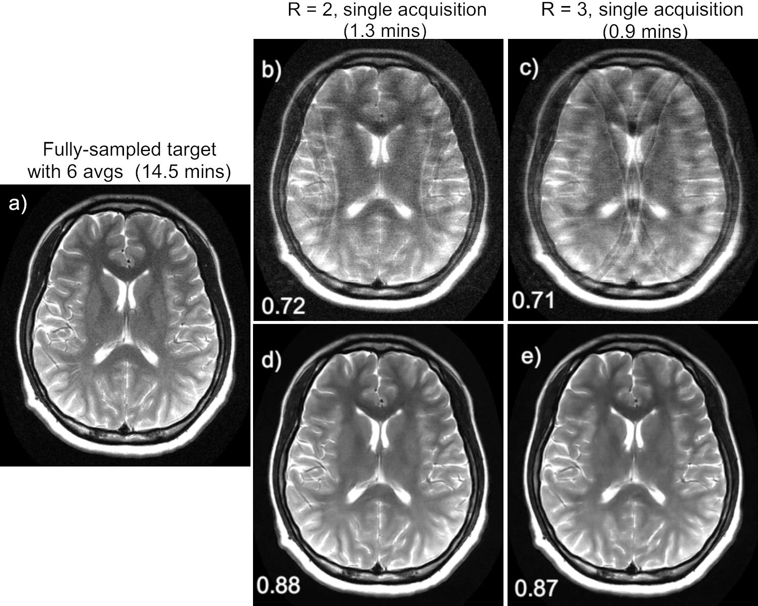
Figure 3. Example result demonstrating combined
denoising and sparse-sampling reconstruction of a T2-weighted brain image. The fully
sampled target with 6 signal averages is shown in (a). The zero-filled
reconstructions for a single acquisition and acceleration factors (R) = 2 and
3, are shown in (b) and (c), respectively. The corresponding VN reconstruction
are shown in (d) and (e). The values indicted in the image are the SSIM values
calculated for the presented slices.