Introduction:

Compressed Sensing (CS) and parallel MRI (pMRI) have been successfully used to accelerate MRI data acquisition [1], [2]. CS requires incoherent sampling, usually achieved by random undersampling of k-space, and sparse reconstruction [3]. pMRI uses more data from an array of receive coils, and also undersamples k-space coherently [4], [5]. Both methods combined synergistically, called here CS-pMRI, can achieve even higher acceleration rates. However, there are not many studies regarding changes in the sampling pattern (SP) for this combined problem. It is also unknown if the SP is dependent on the particular reconstruction method.
Here, we propose an algorithm to learn a good SP from given data and reconstruction method, similarly to [6], but with CS-pMRI images. We focus on T1ρ-weighted images of human knee joint when sparse and low rank reconstructions are utilized [7]. Our preliminary results show that the learning-based SP is superior to others such as Poisson disk [8] and variable density [9] for human knee joint.

Methods:

The CS and low rank (LR) reconstruction [7], [10] is given by:
$$\hat{\mathbf{x}}=\arg\min_\mathbf{x} \left( ||\mathbf{m}- S_ΩFC \mathbf{x}||_2^2+λP(\mathbf{x}) \right)\approx R(\mathbf{m},Ω).$$
Here $$$\mathbf{x}$$$ represents the 2D+time images, of size $$$N_x\times N_y \times N_t$$$ (in our experiments this is $$$128 \times 64 \times 10$$$) which denotes vertical $$$N_x$$$ and horizontal $$$N_y$$$ sizes and time $$$N_t$$$. $$$\mathbf{m}$$$ is the undersampled multicoil k-t-space data. $$$C$$$ denotes the coil sensitivities transform, which maps $$$\mathbf{x}$$$ into multicoil-weighted images of size $$$N_x \times N_y \times N_t \times N_c$$$, with number of coils $$$N_c$$$. $$$F$$$ represents the spatial FFTs, which are $$$N_t \times N_c$$$ repetitions of the 2D-FFT, $$$S_Ω$$$ is the sampling function using SP $$$Ω$$$ (same for all coils) and $$$λ$$$ is the regularization parameter, see details in [7]. The SP contains the k-t-space points to be sampled; it can be displayed as a binary mask with dimensions $$$N_k=N_x \times N_y \times N_t$$$, as shown in Figures 2 to 5. The regularization functions considered are: $$$l_1$$$-norm, as $$$P(x)=||Tx||_1$$$, where $$$T$$$ is the spatiotemporal finite differences (STFD); and low rank (LR), using nuclear-norm of $$$\mathbf{x}$$$ (reshaped as a matrix), given by $$$||\mathbf{x}||_*$$$. We use the iterative algorithm MFISTA-VA [11], to obtain $$$R(\mathbf{m},Ω)$$$, that approximates the above minimization.
Our proposal is similar to [6], but using:
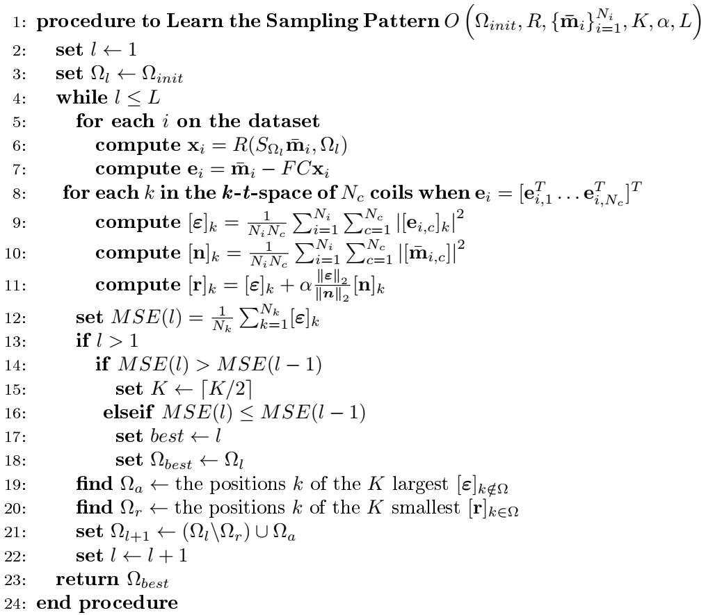
$$\hat{Ω}=\arg\min_Ω\sum_{i=1}^{N_i}||\bar{\mathbf{m}}_{i} –FCR(S_Ω\bar{\mathbf{m}}_{i},Ω)||_2^2 \approx O\left(Ω_{init},R, \{\bar{\mathbf{m}}_{i} \}_{i=1}^{N_i},K,\alpha,L \right).$$

$$$N_i$$$ is the number of images used for learning. We use fully-sampled pMRI data $$$\bar{\mathbf{m}}_{i}$$$, of size $$$N_x \times N_y \times N_t \times N_c$$$ (size $$$128 \times 64 \times 10 \times 15$$$ in the experiments), and $$$O\left(Ω_{init},R, \{\bar{\mathbf{m}}_{i} \}_{i=1}^{N_i},K,\alpha,L \right)$$$ is the algorithm described in Figure 1. Note that the error, denoted by $$$\mathbf{e}_i=[\mathbf{e }_{i,1}^T \ldots \mathbf{e}_{i,N_c}^T ]^T$$$ in the algorithm, is evaluated in the fully-sampled multicoil k-t-space, where $$$\mathbf{e }_{i,c}$$$ is the k-t-space error for the coil $$$c$$$, and $$$i$$$ represent the index of the image in the training set. It is assumed only a fixed fraction of the k-t-space points belongs to $$$Ω$$$, where the acceleration factor (AF) is the ratio of the total number of points to the number of samples. The optimization finds the k-t-space points to be sampled in order to have the approximately best results from the given reconstruction method and dataset.

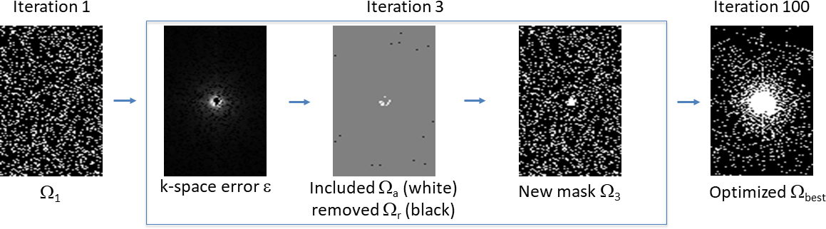
This combinatorial problem is solved by $$$L$$$ iterations (90 in the experiments) of the proposed algorithm, as described in Figure 1, instead of using slow greedy approaches [6]. At each iteration $$$l$$$, it searches among the k-t-space points for the K elements with the largest mean squared error $$$\boldsymbol{\varepsilon}$$$ and smallest regularized error $$$\mathbf{r}$$$ to decide which points should be included and removed, as described in Figure 1 and illustrated in Figure 2. The parameters used in the experiments are: initial $$$K=$$$410, and $$$\alpha=$$$0.1. The proposed algorithm can be applied to any initial SP. We used $$$N_i=$$$40 for training and a validation set with 12 images that are not in the training set.

Results and Discussion:

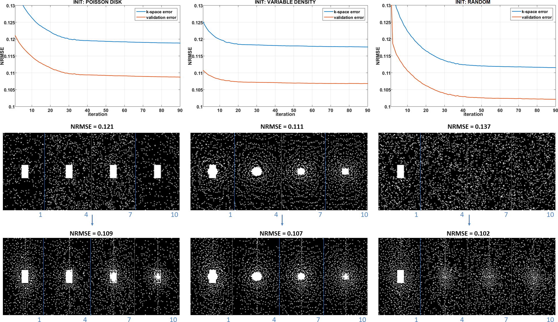
Figure 3 shows the results with different initial SP. One can see that the algorithm converges to different results. This is expected since there is no guarantee of convexity or uniqueness of the optimized SP. However, the quality of the optimized patterns, measured by normalized root mean squared error (NRMSE) of the whole image in the validation set, is always better than the initial patterns.
In Figure 4 the optimized SP for different regularization functions used in $$$R(S_Ω\bar{\mathbf{m}}_{i},Ω)$$$ are shown, one can also note that the optimized SP are different, even with the same initial guess. This difference is also expected since different reconstruction methods recover the missing k-t-space points differently.
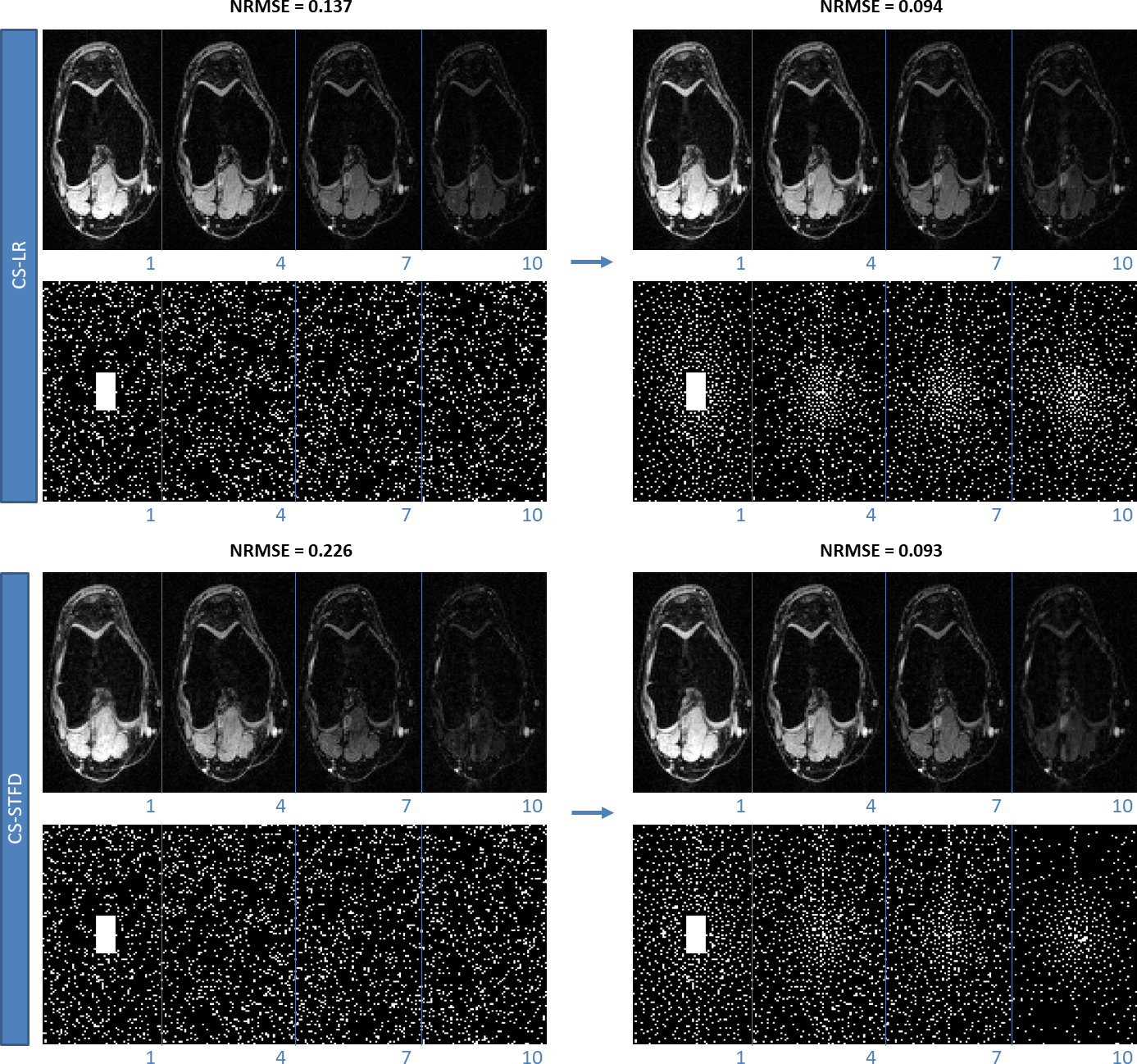
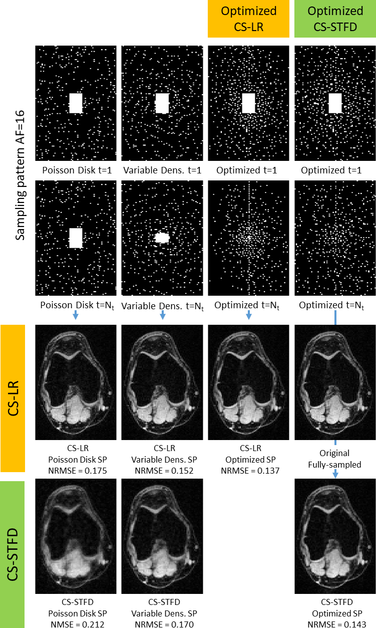
In Figure 5, we show some visual results and NRMSE for AF=16. The NRMSE improvements ranged from 10.3% to 38.8% in the validation images.

Conclusion:

The proposed learning-based method is able to find a better SP considering the reconstruction algorithm and the given data. In this work, we have demonstrated this for the human knee joint, but the proposed approach is generalizable to many other MRI applications involving accelerated CS-pMRI data. The SP for a specific AF can be optimized, for improving the efficiency of MRI data acquisition and reconstruction.

Acknowledgements

This work was supported in part by NIH grants R01-AR067156, and R01-AR068966 and was performed under the rubric of the Center for Advanced Imaging Innovation and Research (CAI2R, www.cai2r.net) an NIBIB Biomedical Technology Resource Center (NIH P41 EB017183).