3451
MRI Below the Noise Floor1New York University School of Medicine, New York, NY, United States, 2Microstructure Imaging INC, New York, NY, United States
Synopsis
We develop random matrix theory (RMT)-based MRI image reconstruction able to increase SNR by up to 10-fold, and to radically increase resolution for routine clinical acquisitions. RMT offers an objective criterion for separating signal from noise across all coils, voxels and MRI contrasts, by utilizing the redundancy in MRI measurements. We demonstrate RMT on a 0.8x0.8x0.8 mm3 neuro exam that includes a series of multiple T2w, T1w, diffusion, and fMRI images on a 3T clinical scanner. RMT can serve as a paradigm for reconstructing multiple contrasts, enhancing image quality for low-field scanners, increasing MR value, and improving biomarker precision.
Introduction
The signal-to-noise ratio (SNR) defines MR image quality and fundamentally limits the MRI resolution. Here, we unlock an untapped reserve for an order-of-magnitude SNR increase. We employ random matrix theory (RMT)1-5 to develop a noise-removing image reconstruction methodology able to recover the signal from below the noise floor, by utilizing the information across multiple coils, voxels and MRI contrasts. The resulting clinical 3T neuro protocol achieves $$$0.8\times0.8\times0.8$$$mm resolution for fMRI, advanced diffusion (dMRI), $$$T_1$$$ and $$$T_2$$$.Methods
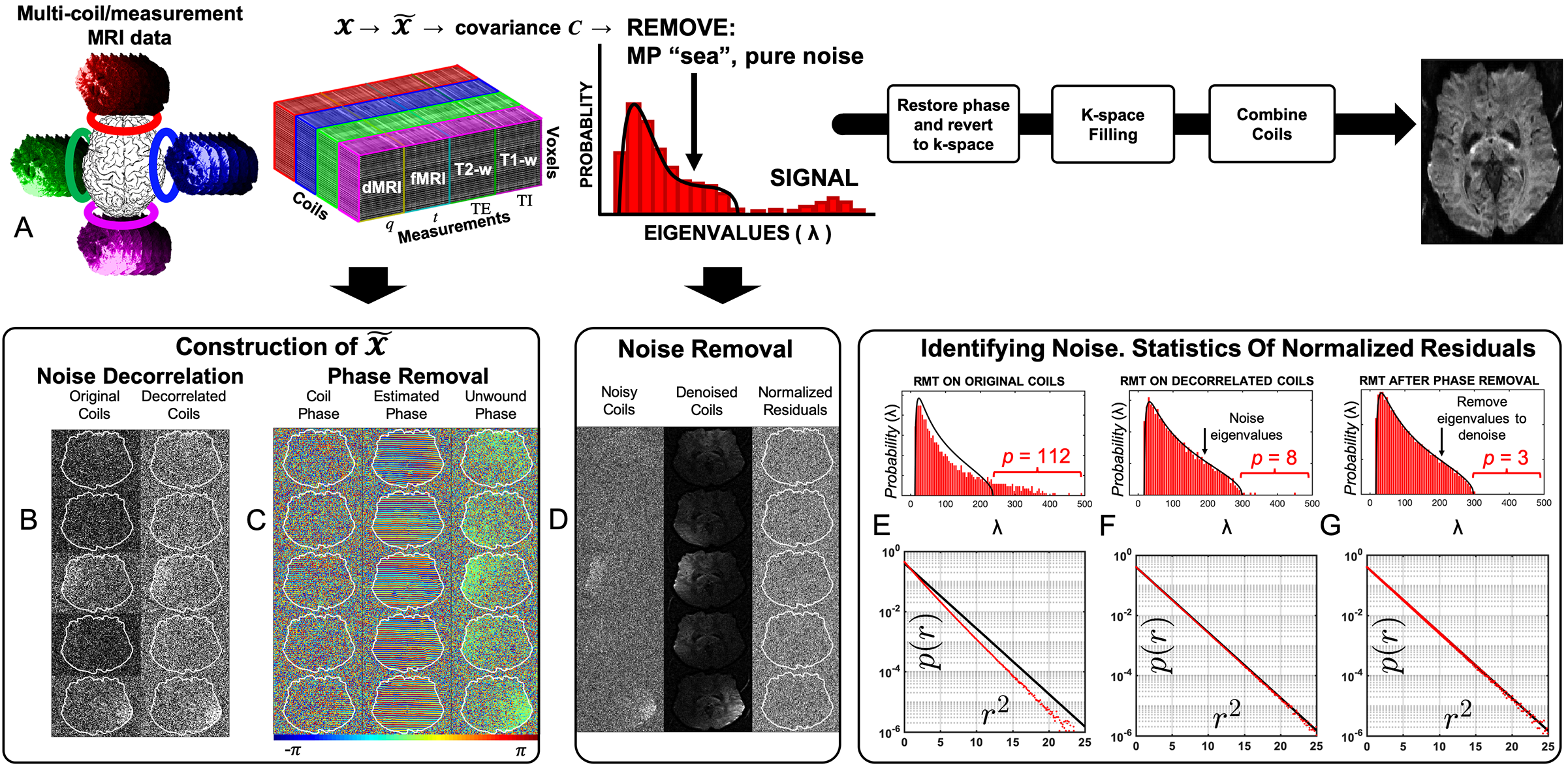
We propose to utilize the redundancy in measuring the tissue of interest from multiple vantage points, Fig.1. Including different rf coils, MRI measurements (e.g., anatomical, diffusion and functional), and adjacent voxels. This redundancy allows us to gain SNR in each of $$$M\sim100$$$ distinct measurements almost by the same $$$\sqrt{M}$$$ as if we were averaging over the same measurement $$$M$$$ times.RMT identifies pure-noise principal components $$$\lambda$$$ in a redundant measurement, i.e., when it has a small number $$$P$$$ of significant components relative to the size of the $$$N\,\times\,M$$$ data-matrix $$$X$$$. While thermal noise makes $$$X$$$ full-rank, in the limit $$$N,M\to\infty$$$ the pure-noise components are distributed according to the Marchenko-Pastur (MP) distribution3$$p_\gamma (\lambda)=\frac{\sqrt{(\lambda_+-\lambda)(\lambda-\lambda_-)}}{2\pi\gamma\sigma^2\lambda},\,\,\,\lambda_-<\lambda<\lambda_+\,\,\,\,\,(1)$$Here $$$\sigma$$$ is the noise level, $$$\gamma=M/N$$$, and $$$\lambda_\pm=\sigma^2(1\pm\sqrt{\gamma})^2$$$ are the boundaries of MP distribution. We identify and remove the contribution (1) to the PCA spectrum of $$$X$$$.
Contrary to previous approaches6,7, we start from a rank-3 data matrix$$$\,\mathcal{X}$$$: coils$$$\,\times\,$$$measurements ($$$T_2w,\,T_1w$$$, dMRI, fMRI, etc)$$$\,\times\,$$$voxels, size $$$N_c\times N_m\times N_x$$$, which we reshape to size $$$M\,\times\,N$$$ to make it closest to a square, $$$M\,\sim\,N$$$. Redundancy in coils and measurements enables a sharp separation between pure-noise and signal, and lets us minimize the size $$$N_x\sim27-45$$$ of the local spatial patch.
The distribution (1) relies on uncorrelated noise. Hence, we apply RMT after coil noise decorrelation and phase-unwinding, and before k-space filling, since standard k-space filling techniques8-12 make noise correlated13.
Experiments were performed on a 3T Siemens Prisma system with a 20-channel head/neck coil, of which 16 elements were enabled. After RMT denoising, standard reconstruction steps were applied, including adaptive-combine14.
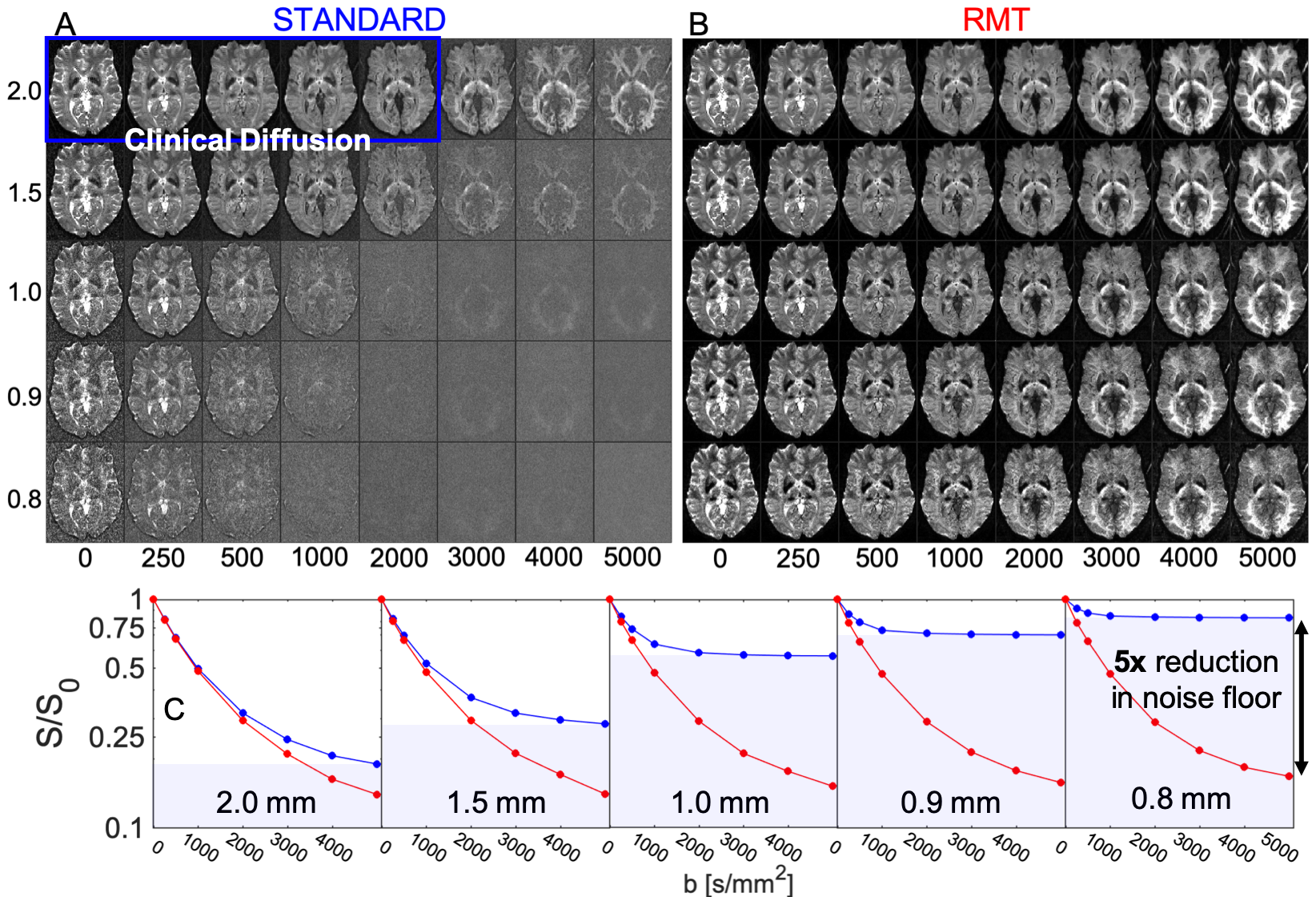
- Diffusion at different resolutions (Fig.1-3): A 3-slice brain slab from a 31 y/o female volunteer was acquired with different isotropic resolutions [0.8,0.9,1.0,1.5,2.0] mm (original SNR = [2.5,3.1,4.0,7.9,14.9] at $$$b=0$$$), $$$T_R=3$$$s,$$$\,T_E=132$$$ms, with 8 $$$b$$$-shells [0,250,500,1000,2000,3000,4000,5000] along [1,6,6,12,20,30,30,40] directions, respectively. Scan time was 7min per resolution.
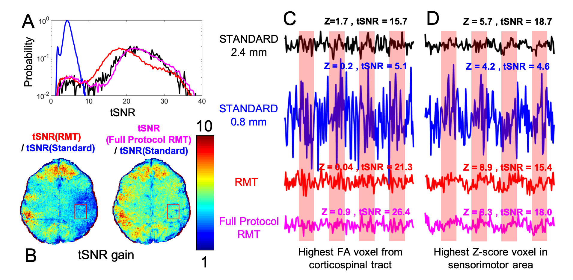
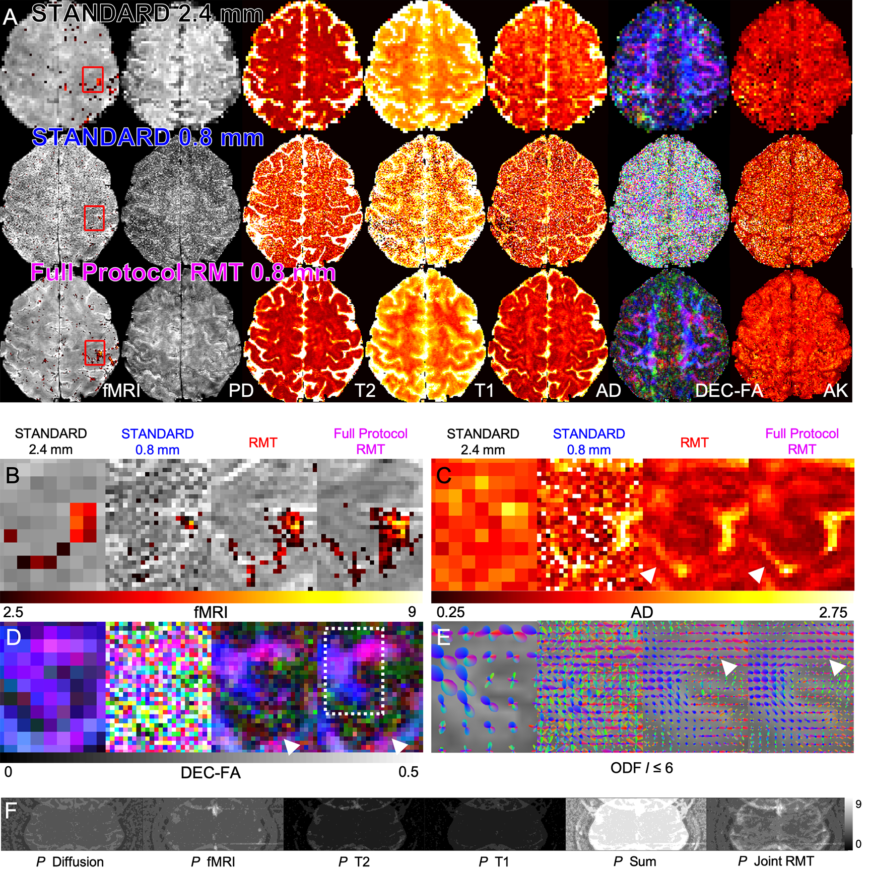
- Multimodal protocol at $$$0.8\times0.8\times0.8$$$mm resolution (Fig.4-5): A 5-slice segment of the brain from a 28 y/o male volunteer with various contrasts was acquired through the hand knob of the precentral gyrus, using GRAPPA10 $$$R=2$$$, pFourier 6/8 with POCS (original SNR 3.31 at $$$b=0$$$). Total scan time was 12:30. There were $$$N_m=256$$$ total measurements [70 SE diffusion ($$$10 b = 0, 20 b = 1000, 40 b = 2000$$$), 13 SE IR images for $$$T_1$$$ mapping ($$$T_R=4000\,$$$ms, $$$T_E=77$$$, $$$BW = 1125.2$$$ Hz/pix, $$$T_I=[33-2000]$$$), 13 SE images for $$$T_2$$$ mapping ($$$T_R=4000$$$,$$$\,T_E=[80-200]$$$), and 160 GE images for a right index finger tapping fMRI ($$$T_R=1000$$$ms, $$$T_E=39$$$ms, FA$$$=62^\circ$$$, using 8 on/off 20s epochs). The standard protocol at 2.4 mm resolution was generated by using 1/3 of the k-space in each dimension.
All images were aligned using TOPUP15+EDDY16,17. The z-scores to measure cortical activation were determined after motion correction, slice timing correction, brain extraction, high-pass temporal filtering, and BOLD modeling using FSL-FEAT18 [Fig.4,5]. 36 SE images for $$$b=0$$$ were used to calculate proton density $$$S_0$$$, $$$T_1$$$ and $$$T_2$$$ times, via:$$S(T_I,T_R,T_E)=S_0[1-2e^{-T_I/T_1}+e^{-T_R/T_1}]e^{-T_E/T_2}\,\,\,\,\,\, (2)$$Diffusion images were processed for WLLS diffusion tensor/kurtosis19 estimation. Fiber orientation distributions were estimated using mrtrix320 for up to $$$l=6$$$ spherical-harmonics order.
Results & Discussion
In Fig.1, we summarize RMT-reconstruction, and demonstrate perfectly white-noise residuals down to $$$5\sigma$$$ (Fig.1G).Fig.2: RMT recovers high-$$$b$$$ diffusion images from under the noise floor, down to $$$0.8\times0.8\times0.8$$$ voxels, yielding at least $$$5\times$$$ noise reduction.
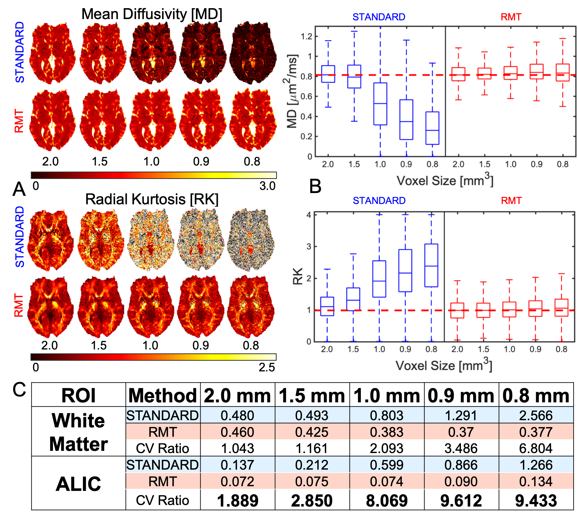
Fig.3: RMT provides up to $$$10\times$$$ precision increase for mean diffusivity. Moreover, RMT successfully removes the noise-floor bias in both MD and RK, where mean values at high and low match.
Fig.4: RMT increases temporal SNR over $$$5\times$$$ for task-fMRI, enabling unprecedented $$$0.8\times0.8\times0.8$$$ voxels at 3T. The fMRI time-courses (normalized by their mean values) show clear noise reduction, with the full-protocol RMT reconstruction yielding the highest gain in precision.
Fig.5: RMT reaches its fullest potential on a multimodal neuro protocol, where information is shared between contrasts. Indeed, the number $$$P$$$ of information-carrying components outside of the distribution (1) after full-protocol-RMT is notably smaller than the sum of $$$P$$$ from RMT on individual modalities (fMRI, diffusion, etc).
Conclusions & Outlook
- By objectively identifying the low-rank structure12,21-25 across all MRI contrasts/voxels/coils, RMT reconstruction unlocks an untapped $$$\sim10\times$$$ SNR reserve, essentially for free.
- RMT prompts acquiring all clinically necessary contrasts with the same highest possible resolution and jointly denoise all of them, whereby each measurement alone would drown in noise.
- RMT is complementary to hardware improvements (high field, multi-coils, strong gradients). It can further improve image quality for low-field scanners reducing cost and increasing MRI value.
- RMT has potential to enhance the performance of modern acquisitions and reconstruction algorithms, and increase accuracy and precision of imaging biomarkers lowering sample sizes for human studies.
- RMT reveals information content of MRI, and serves as a paradigm to combine multiple contrasts, without relying on priors or training data.
Acknowledgements
We thank Daniel Sodickson and Kawin Setsompop for discussions. This work was supported by the NIH under awards number R01NS088040 (NINDS) and R01EB027075 (NIBIB), and by the Center of Advanced Imaging Innovation and Research (CAI2R, www.cai2r.net), a NIBIB Biomedical Technology Resource Center: P41 EB017183.References
1. Wigner EP. On the Distribution of the Roots of Certain Symmetric Matrices. Annals of Mathematics 1958;67:325-7.
2. Dyson FJ. Statistical Theory of the Energy Levels of Complex Systems. I. Journal of Mathematical Physics 1962;3:140-56.
3. Marchenko VA, Pastur LA. Distribution of eigenvalues for some sets of random matrices. Mathematics of the USSR-Sbornik 1967;1:457.
4. Baik J, Ben Arous G, Peche S. Phase transition of the largest eigenvalue for nonnull complex sample covariance matrices. Ann Probab 2005;33:1643-97.
5. Johnstone IM. High Dimensional Statistical Inference and Random Matrices. arXiv Mathematics e-prints2006.
6. Veraart J, Novikov DS, Christiaens D, Ades-Aron B, Sijbers J, Fieremans E. Denoising of diffusion MRI using random matrix theory. Neuroimage 2016;142:394-406.
7. Cordero-Grande L, Christiaens D, Hutter J, Price AN, Hajnal JV. Complex diffusion-weighted image estimation via matrix recovery under general noise models. NeuroImage 2019;200:391-404.
8. Feinberg DA, Hale JD, Watts JC, Kaufman L, Mark A. Halving MR imaging time by conjugation: demonstration at 3.5 kG. Radiology 1986;161:527-31. 9. Pruessmann KP, Weiger M, Scheidegger MB, Boesiger P. SENSE: sensitivity encoding for fast MRI. Magn Reson Med 1999;42:952-62.
10. Griswold MA, Jakob PM, Heidemann RM, et al. Generalized autocalibrating partially parallel acquisitions (GRAPPA). Magn Reson Med 2002;47:1202-10.
11. Lustig M, Donoho D, Pauly JM. Sparse MRI: The application of compressed sensing for rapid MR imaging. Magnetic Resonance in Medicine 2007;58:1182-95.
12. Uecker M, Lai P, Murphy MJ, et al. ESPIRiT--an eigenvalue approach to autocalibrating parallel MRI: where SENSE meets GRAPPA. Magn Reson Med 2014;71:990-1001.
13. Sprenger T, Sperl JI, Fernandez B, Haase A, Menzel MI. Real valued diffusion-weighted imaging using decorrelated phase filtering. Magn Reson Med 2017;77:559-70.
14. Walsh DO, Gmitro AF, Marcellin MW. Adaptive reconstruction of phased array MR imagery. Magn Reson Med 2000;43:682-90.
15. Andersson JLR, Skare S, Ashburner J. How to correct susceptibility distortions in spin-echo echo-planar images: application to diffusion tensor imaging. NeuroImage 2003;20:870-88. 16. Andersson JL, Sotiropoulos SN. An integrated approach to correction for off-resonance effects and subject movement in diffusion MR imaging. Neuroimage 2016;125:1063-78.
17. Andersson JLR, Graham MS, Drobnjak I, Zhang H, Campbell J. Susceptibility-induced distortion that varies due to motion: Correction in diffusion MR without acquiring additional data. NeuroImage 2018;171:277-95.
18. Woolrich MW, Ripley BD, Brady M, Smith SM. Temporal autocorrelation in univariate linear modeling of FMRI data. Neuroimage 2001;14:1370-86.
19. Jensen JH, Helpern JA, Ramani A, Lu H, Kaczynski K. Diffusional kurtosis imaging: The quantification of non-gaussian water diffusion by means of magnetic resonance imaging. Magnetic Resonance in Medicine 2005;53:1432-40.
20. Tournier JD, Smith R, Raffelt D, et al. MRtrix3: A fast, flexible and open software framework for medical image processing and visualisation. NeuroImage 2019;202:116137.
21. Sengupta, A. M. & Mitra, P. P. Distributions of singular values for some random matrices.Physical Review E60, 3389–3392(1999).
22. Pedersen, H., Kozerke, S., Ringgaard, S., Nehrke, K. & Kim,W. Y. k-t PCA: Temporally constrained k-t BLAST reconstruction using principal component analysis.Magnetic Resonance in Medicine 62, 706–716 (2009).
23. Petzschner, F. H., Ponce, I. P., Blaimer, M., Jakob, P. M. &Breuer, F. A. Fast MR parameter mapping using k-t principal component analysis.Magnetic Resonance in Medicine 66, 706–716 (2011).
24. Otazo, R., Candes, E. & Sodickson, D. K. Low-rank plus sparsematrix decomposition for accelerated dynamic MRI with separation of background and dynamic components.Magnetic Resonance in Medicine 73, 1125–1136 (2015).
25. Zhao, B.et al.Accelerated MR parameter mapping with low-rank and sparsity constraints.Magnetic Resonance in Medicine 74, 489–498 (2015).
Figures