Introduction

Chemical exchange saturation transfer (CEST) MRI enables detection of tissue metabolites but requires the acquisition of a full Z-spectrum¹ for quantitative measurement. When gated for cardiac imaging, scan times routinely exceed one hour. While acquisition acceleration has been proposed using compressed sensing and parallel imaging^2,3, this work examines the use of multiscale low rank (MSLR) matrix decomposition to further exploit signal sparsity in the Z-spectrum domain⁵ for reconstruction of retrospectively subsampled cardiac-CEST data.

Methods

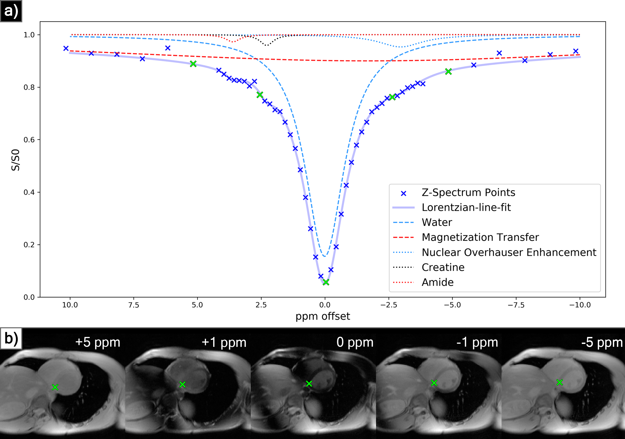
MSLR has been utilised to perform computationally efficient reconstruction of non-gated dynamic MRI⁶ while preserving dynamic contrast effects. Similarly to how there exists high spatio-temporal correlation in dynamic MRI, in CEST MRI there is high structural similarity between Z-spectra acquisitions (fig. 1b), implying the existence of a compressed representation in the Z-domain.This constrains reconstruction as follows:

The acquired image sequence is proposed to be represented by:
$$\mathbf{x}_{z}=\sum_{j=1}^{J} \mathcal{M}_{j}\left(\mathbf{L}_{j} \mathbf{R}_{j}[z]^{H}\right)$$Where $$$\mathbf{x_z}$$$ is a CEST acquisition image at offset index $$$z$$$, represented by a summation over $$$j \in [1, ..., J]$$$ block scales. Here, $$$\mathbf{L_{j}}$$$ are block spatial bases, $$$\mathbf{R_{j}}[z]$$$ are Z-spectrum bases, and $$$\mathcal{M}_{j}$$$ embeds an input block matrix into the acquired image.

The resultant parallel k-space acquisitions $$$y_{zc}$$$ at offset $$$z$$$ and channel $$$c$$$ are modeled by:$$\mathbf{y}_{zc}=\mathbf{F}_{z} \mathbf{S}_{c} \sum_{j=1}^{J} \mathcal{M}_{j}\left(\mathbf{L}_{j} \mathbf{R}_{j}[z]^{H}\right)+\mathbf{w}_{zc}$$Where $$$\mathbf{F}_z$$$ is the Fourier sampling operator, $$$\mathbf{S}_c$$$ is the sensitivity map operator, and $$$\mathbf{w}_{zc}$$$ is white Gaussian noise.

The objective is then to find optimal bases $$$\mathbf{L_{j}}$$$ and $$$\mathbf{R_{j}}[z]$$$ which minimize:$$f(\mathbf{L}, \mathbf{R})=\sum_{z=1}^{Z} \frac{1}{2}\left\|\mathbf{y}_{z c}-\mathbf{F}_{z} \mathbf{S}_{c} \sum_{j=1}^{J} \mathcal{M}_{j}\left(\mathbf{L}_{j} \mathbf{R}_{j}[z]^{H}\right)\right\|_{2}^{2}+\sum_{j=1}^{J} \frac{\lambda_{j}}{2}\left(\left\|\mathbf{L}_{j}\right\|_{F}^{2}+\left\|\mathbf{DR}_{j}\right\|_{F}^{2}\right)$$Where the left side of the equation is the total reconstruction error for acquisitions $$$z \in [1, …, Z] $$$, and the right is a regularization factor, weighted by $$$\lambda_j$$$, which requires the manual selection of one global regularization parameter $$$\lambda$$$. Here, an optional transform operator $$$\mathbf{D}$$$ can be applied to the Z-spectrum bases. We use finite differences to promote smoothness both spatially and along the Z-spectrum domain.

The method was tested on cardiac CEST scans acquired on a 3T Siemens Trio scanner (Siemens Medical Systems, Erlangen, Germany) from 10 healthy volunteers with IRB approval and informed consent, with no history of cardiovascular disease, diabetes, or smoking, aged 20-37. A scan consisted of 52-56 segmented echo planar gradient echo acquisitions, each corresponding to a point on the produced Z-spectrum. Parameters as follows: FOV = 300 x 253mm, spatial resolution = 1.56 x 1.56mm, slice thickness = 8mm, TR = 4.7ms, TE = 2.59ms, and FA = 25°, timed to end-diastole.

Sensitivity maps $$$\mathbf{S}_c$$$ were calculated via JSENSE reconstruction⁷ on low-resolution calibration data, and the objective function $$$f(\mathbf{L}, \mathbf{R})$$$ was optimized using stochastic gradient descent across acquisitions⁸. The data were retrospectively accelerated with variable density random undersampling⁹, with a central k-space fraction of 0.1, 0.08, 0.07, and 0.06 for acceleration factors 2, 4, 6, and 8 respectively. To separate CEST effects, water saturation, magnetization transfer (MT), and nuclear overhauser effect (NOE), Z-spectra were analysed with a five pool lorentzian-line-fit¹⁰ (fig 1a). This fit was achieved by nonlinear least squares optimization, with initial parameters defined by known physical properties of the CEST agents and byproduct effects.

Results

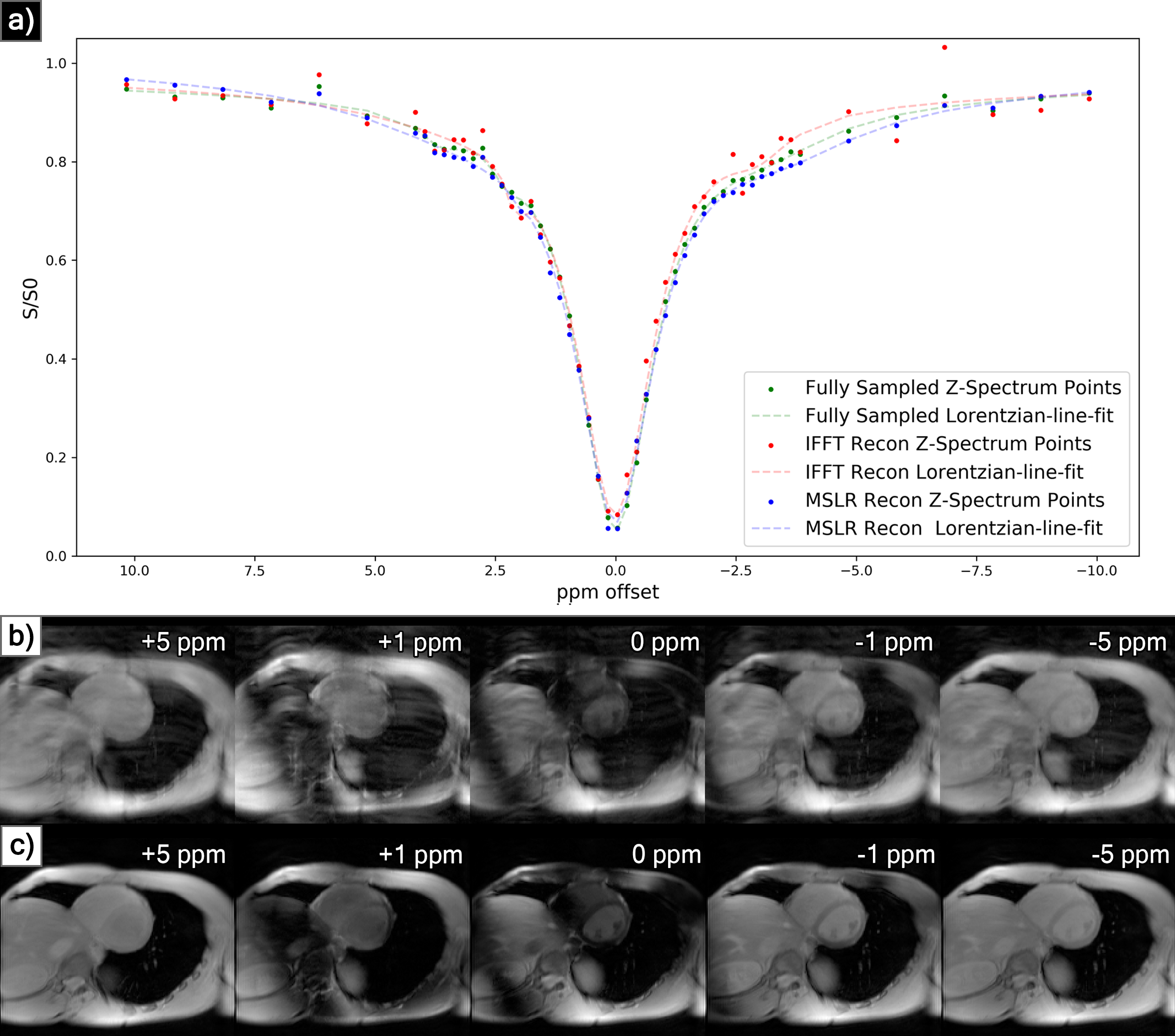
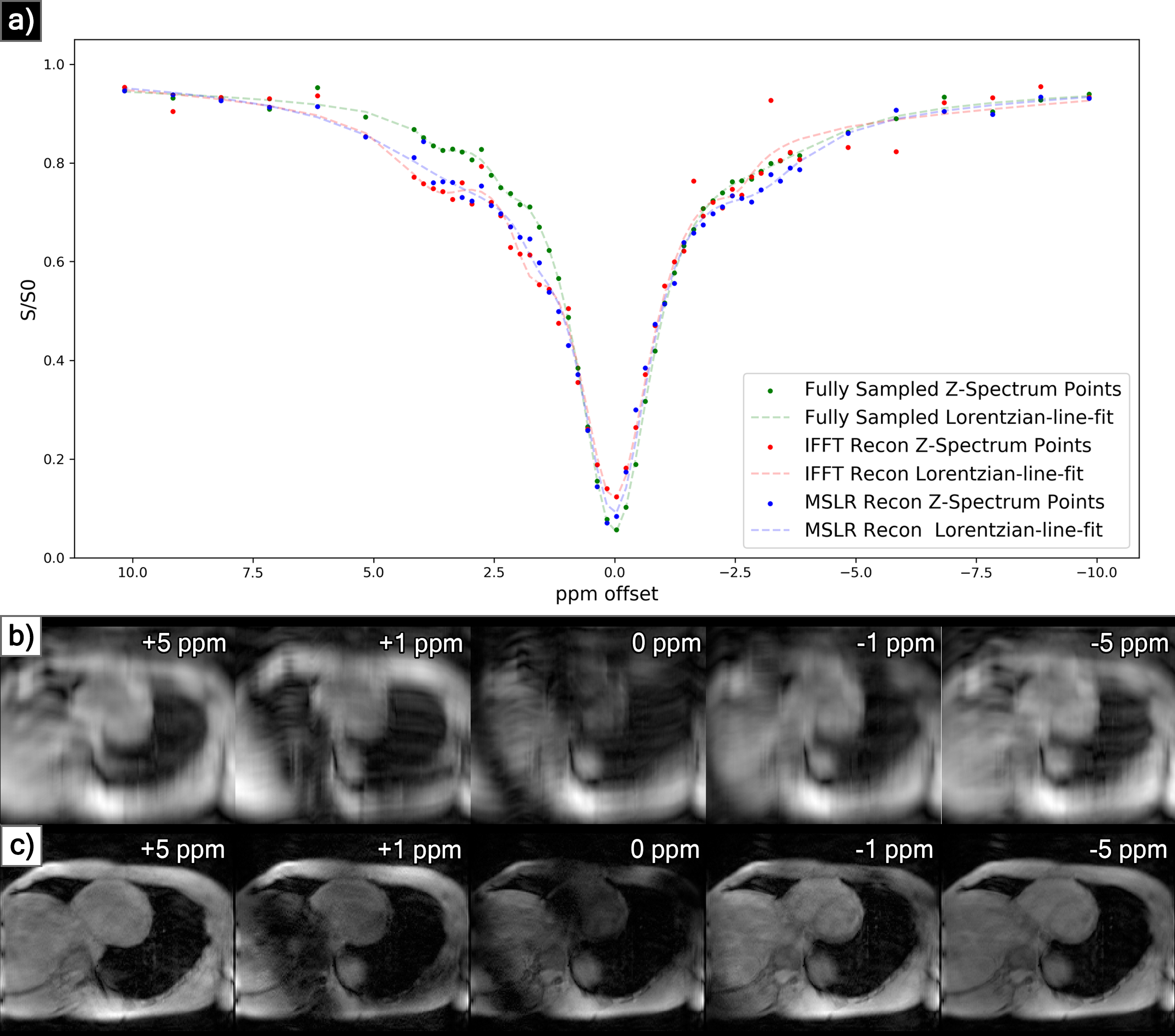
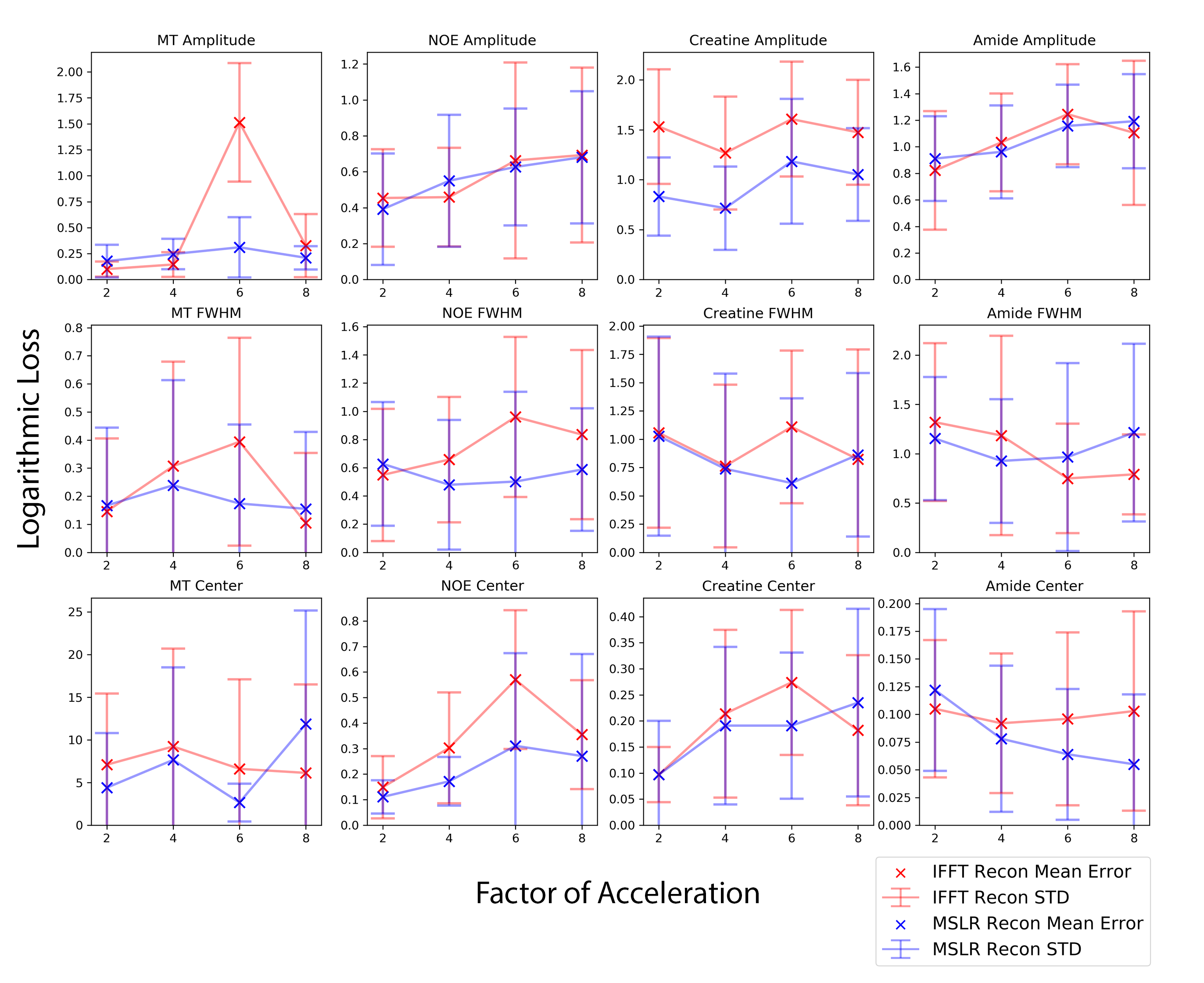
At acceleration factors of 2 and 4, MSLR reconstruction recovers nearly all cardiac structure (figure 2b and 3b), while preserving the CEST effect and scan features such as phase dispersion bands from field inhomogeneity. At acceleration factor 8, to ensure reconstruction of cardiac tissue structure and minimize smoothing of CEST effects, regularization is heavily reduced, with $$$\lambda$$$ on the order of $$$10^{-8}$$$. This leads to high-frequency spatial and temporal artifacts appearing in scan reconstruction (figure 4b); which deteriorate the produced Z-spectra to below the quality observed from direct zero-filled IFFT reconstruction (figure 4a).

Overall, MSLR reconstruction on retrospectively under-sampled data significantly outperforms zero-filled IFFT in the measure of creatine CEST signal amplitude (figure 5), and shows comparable reconstruction of NOE and amide CEST. Both reconstruction methods show a very high deviation in MT center from fully sampled scans, however the associated Lorentzian has full width at half max (FWHM) magnitudes larger than the other four pools, and the effect of a large shift in its center frequency is minor.

While CEST and NOE amplitudes in the IFFT reconstructions were equally often underestimated and overestimated in scans at varying accelerations, MSLR reconstruction always led to higher calculated amplitudes than the fully-sampled scans.

Discussion

In the MSLR pipeline for dynamic MRI⁶ acquisitions are assumed to be equidistant in time, however when this time domain is converted to act a Z-spectrum domain this assumption does not hold true. As samples along the Z-spectrum are not equally spaced, density correction should be added into the objective function to control changes in contrast during reconstruction. By adding offset-dependent weighting on the finite difference operator $$$\mathbf{D} \rightarrow \mathbf{D}_z$$$ it could be possible to restrict large contrast changes in the CEST and NOE regions while allowing for sharp global changes in contrast around water saturation, leading to a more accurate Lorentzian-line-fit derived for all 5 pools.

References

1. Wu B, Warnock G, Zaiss M, et al. An overview of CEST MRI for non-MR physicists. EJNMMI
2. Phys. 2016;3(1):19. doi:10.1186/s40658-016-0155-22. She H, Greer JS,Zhang S, et al. Accelerating chemical exchange saturation transfer MRI with parallel blind compressed sensing. (2019) Magnetic resonance in medicine, 81(1), 504-513.
3. Heo, Hye‐Young, et al. Accelerating chemical exchange saturation transfer (CEST) MRI by combining compressed sensing and sensitivity encoding techniques. Magnetic resonance in medicine 77.2 (2017): 779-786.
4 .Ong F, Lustig M. Beyond low rank + sparse: Multiscale low rank matrix decomposition. IEEE journal of selected topics in signal processing 10.4 (2016): 672-687.
5. Kwiatkowski G, Kozerke S. Accelerating CEST MRI by Exploiting Sparsity in the Z-Spectrum Domain. In Proceedings of the 27th Annual Meeting of ISMRM, Montreal, QC, Canada.
6. Ong F, Zhu X, Cheng J, et al.Extreme MRI: Large-Scale Volumetric Dynamic Imaging from Continuous Non-Gated Acquisitions. (2019) Submitted to Magnetic Resonance in Medicine as a Full Paper.
7. Ying L, Sheng J. Joint image reconstruction and sensitivity estimation in SENSE (JSENSE). (2007) Magnetic Resonance in Medicine: An Official Journal of the International Society for Magnetic Resonance in Medicine, 57(6), 1196-1202.
8. Robbins H, Monro S. A Stochastic Approximation Method. (1951) The Annals of Mathematical Statistics; 22:400–407.
9. Lustig M, Donoho D, Pauly J.M. Sparse MRI: The application of compressed sensing for rapid MR imaging. (2007) Magnetic Resonance in Medicine: An Official Journal of the International Society for Magnetic Resonance in Medicine, 58(6), 1182-1195.
10. Zaiß M, Schmitt B, Bachert P. Quantitative separation of CEST effect from magnetization transfer and spillover effects by Lorentzian-line-fit analysis of z-spectra. (2011) Journal of magnetic resonance, 211(2), 149-155.