3449
Multi-Component Quantitative T2 Shuffling: Accelerating Myelin Water Imaging by 20-30x1Physics and Astronomy, University of British Columbia, Vancouver, BC, Canada, 2International Collaboration on Repair Discoveries (ICORD), Vancouver, BC, Canada, 3MR Clinical Science, Philips Canada, Markham, ON, Canada, 4Radiology, University of British Columbia, Vancouver, BC, Canada, 5Medicine (Neurology), University of British Columbia, Vancouver, BC, Canada
Synopsis
Multi-component quantitative T2 mapping can provide a range of valuable, in-vivo biomarkers, but is limited by lengthy acquisition times. Here we introduce multi-component quantitative T2 shuffling, a subspace-constrained CS method for reconstructing highly under-sampled multi-component relaxation mapping data using principal components of a temporal basis. We demonstrated reconstruction of myelin water imaging data with simulated under-sampling acceleration factors of ~20-30, which could provide accurate images, higher resolution and fit-to-noise ratios, and improved metric maps in a fraction of the acquisition time.
Introduction
Multi-component quantitative T2 (mcQT2) mapping can characterize water pools present in human tissue. One such technique, myelin water imaging (MWI), provides the myelin water fraction (MWF) metric, one of the most myelin-specific MRI biomarkers available1,2. MWI techniques generally acquire ~50 separate T2 weighted images, necessitating extremely lengthy acquisition times.Compressed sensing3,4 (CS) can exploit a temporal or parameter mapping dimension to facilitate additional under-sampling5. Pivotal work by Huang et al., Tamir et al., and others demonstrated that accounting for signal evolution allows data acquired throughout the echo train to inform image reconstruction6-9 without the blurring induced by alternative methods, such as the GRASE sequence10,11 or fast spin-echo echo-sharing12.
Recently, principal component analysis denoising has been shown to be highly effective at reducing errors in mcQT2 metrics13.
The purpose of this study is to introduce multi-component quantitative T2 shuffling, a subspace-constrained CS method for reconstructing highly under-sampled multi-component relaxation mapping data using principal components of a temporal basis.
Methods
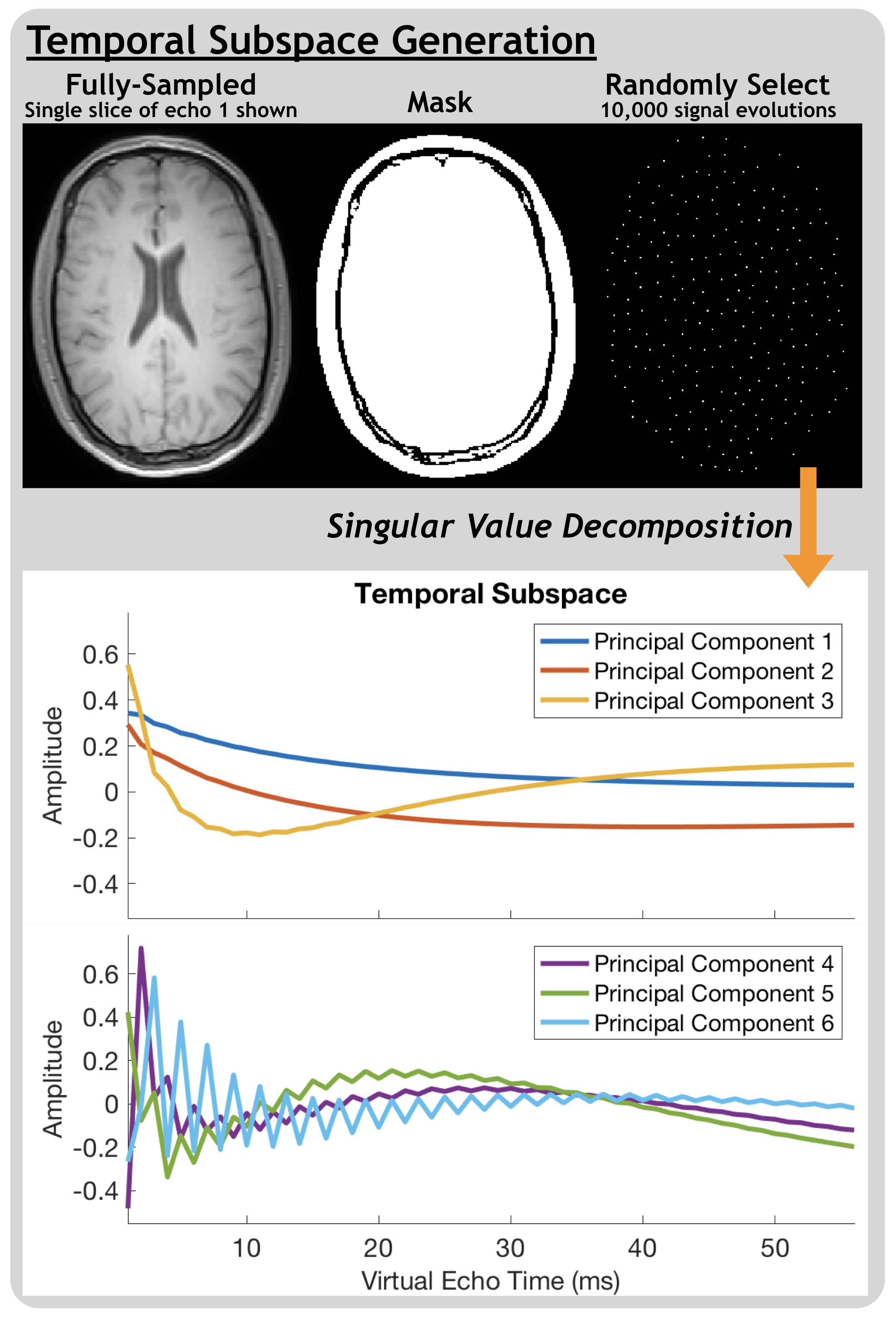
MRI DataA fully-sampled, gold-standard MWI dataset was acquired in 2h:2m:40s for a single healthy volunteer (male, 25 years) with a 3D multi-echo Carr-Purcell-Meiboom-Gill spin-echo sequence (56 echoes, echo spacing 5.7ms, repetition time 1277ms, acquired resolution 1x2x2mm3, field-of-view 230x100x192mm3) at 3T with a 32-channel head coil (Ingenia Elition X, Philips Healthcare, Best, The Netherlands).
To reduce computational demands, k-space data with 8 virtual channels was generated from the fully-sampled dataset and simulated coil sensitivity maps. Retrospective under-sampling was performed for axial slices using variable-density Poisson-disk sampling masks with an elliptical shutter.
mcQT2 Shuffling
10,000 signal evolutions were used to generate a temporal basis set with singular value decomposition, from which principal components were taken to form a temporal subspace (process outlined in Figure 1). Data can be represented in a lifted k-t space as temporal basis set coefficients $$$\alpha = \Phi^Hx$$$. A low-dimensional subspace constraint is applied by taking K principal basis components, where $$$x\approx\Phi_K\Phi^H_Kx$$$, within model error. Extending the CS forward model, the reconstruction problem becomes:
$$\min_{\alpha}\frac{1}{2}\parallel y-MFS\Phi_K\alpha\parallel^2_2+\lambda\parallel T(\alpha)\parallel_1 $$
for sampling mask $$$M$$$, Fourier transform $$$F$$$, coil sensitivity maps $$$S$$$, temporal subspace $$$\Phi_K$$$, regularization $$$\lambda$$$ , and wavelet transform $$$T(\alpha)$$$, solved in Matlab using BART14 with FISTA15.
Analysis
MWI analysis used a regularized non-negative least-squares fitting algorithm with stimulated echo correction16. Fit quality was quantified by fit-to-noise ratio (FNR) maps, calculated for non-negative T2 component amplitudes $$$a_i$$$ as:
$$FNR = \frac{\sum_{i=1}^{nT_2}a_i}{\sqrt{\frac{\sum( residuals^2)}{nEchoes-1}}}$$
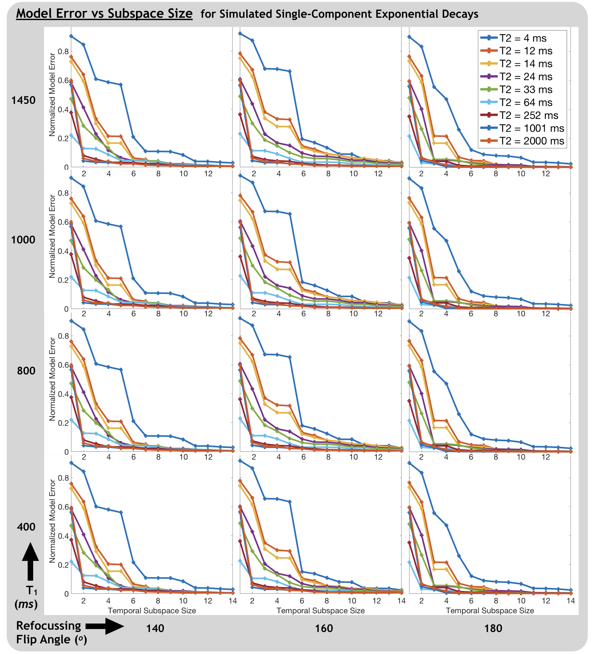
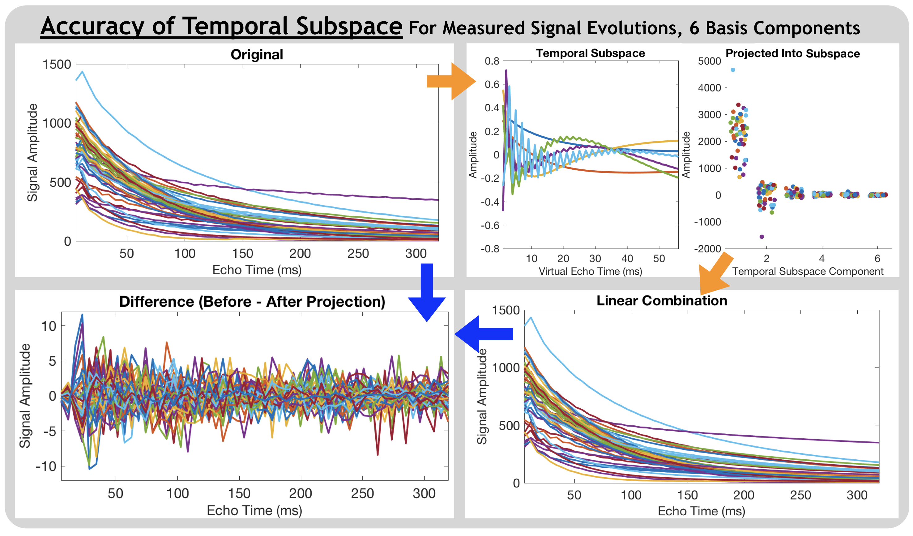
Normalized model error (NME)8 was calculated for single component exponential decays, generated using the extended phase graph algorithm17. Fully sampled images and metric maps were compared to under-sampled mcQT2 shuffling results visually and with normalized mean-square error (NMSE) for a range of subspace sizes, K, and under-sampling acceleration factors, R.
Results and Discussion
Subspace AccuracyInterestingly, without enforcing expectations regarding the number of distinct water pools or their mean T2 values, the first 3 temporal basis components resembled decays with distinct relaxation times (Figure 1). From Figure 2, ~6-8 subspace components were required to flexibly model a wide range of (simulated single-component) signal evolutions with NME of ~0.1 or less. Unsurprisingly, the subspace better models the multi-component relaxation it was designed for (Figure 3). With 6 subspace components, NME for all measured signal evolutions not included in subspace generation was 0.01.
Temporal Denoising
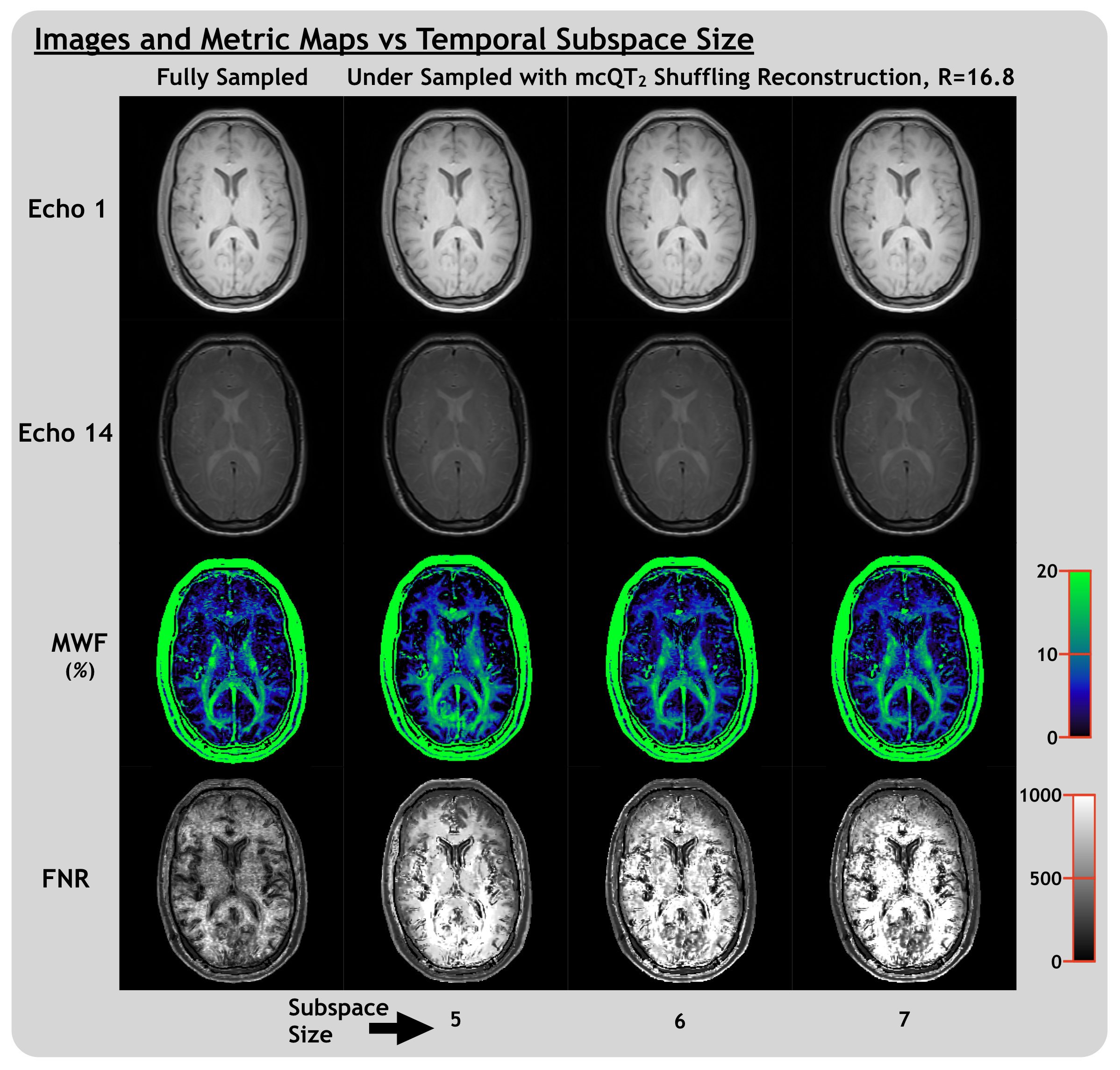
Figure 4 demonstrates the temporal denoising effect the subspace constraint had on images and metric maps, influenced by reconstructing with larger or smaller values of K. For K<6, MWF map features are lost and for K>6, noise-like features, present in the fully-sampled MWF map, begin to be re-introduced. The value of K must be carefully chosen to balance the trade-off between noise and bias8. Ideally, K would be derived objectively for each dataset using the Marchenko-Pastur distribution18 or an alternative method.
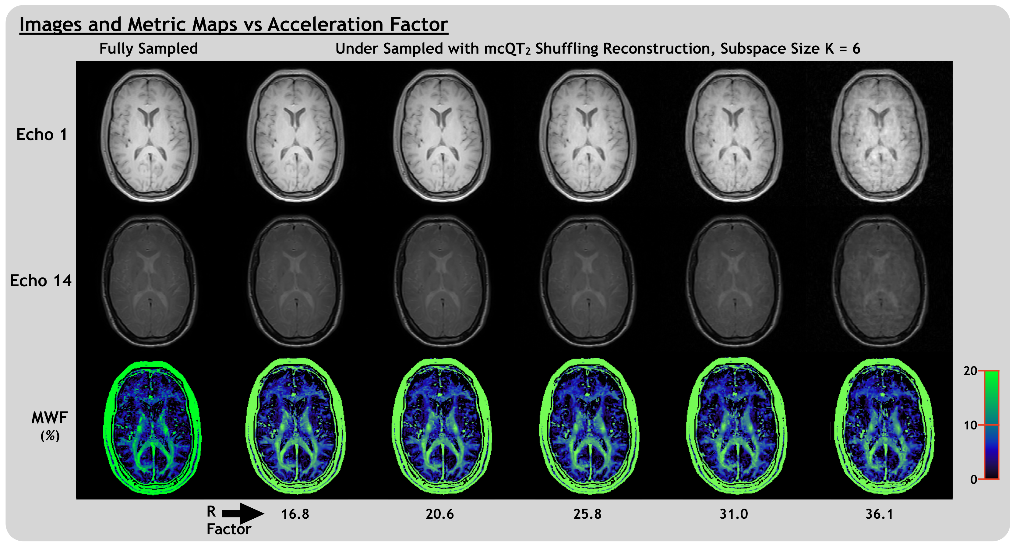
Image and Metric Quality
For mcQT2 shuffling with K=6 and R=25.8 (for which acquisition time would be 4m:45s), mean FNR was 623, compared to 370 for fully-sampled data. For K=6 and R<~30, MWF maps remained qualitatively similar (Figure 5) with relatively stable NMSE (R|NMSE: 5.2|0.045, 10.3|0.045, 16.8|0.050, 20.6|0.052, 25.8|0.063, 31.0|0.084, 36.1|0.119). NMSE of all echo images was <0.005 for R<=31.0, 0.013 for R=36.1. The mean MWF was robust to acceleration, differing from the fully-sampled mean by 0.2% absolute MWF units or less for all R.
Stimulated echo correction is essential for accurate MWI analysis, which may explain why including up to at least K=6 (which appears to be a stimulated echo amplitude modulation) was essential for recovering accurate MWF maps.
Further Considerations
For various mcQT2 mapping techniques, achievable acceleration factors will largely depend on the number of spatial and temporal samples (phase-encode steps and echo times). For example, increased benefits can be expected for techniques with longer echo trains, such as luminal water imaging of prostate19.
The acquisition has been implemented, and preliminary data acquired, with a modified version of the PROUD patch for pseudo-spiral 4D-flow MRI20,21. Each phase-encode value at each echo time can be uniquely specified, which allows for flexible, temporally-incoherent sampling schemes.
Conclusion
mcQT2 shuffling can reconstruct myelin water imaging data with under-sampling acceleration factors of ~20-30, providing accurate images, higher resolution and fit-to-noise ratio, and improved metric maps in a fraction of the acquisition time.Acknowledgements
Adam Dvorak is in receipt of a 4-Year Doctoral Fellowship from the University of British Columbia. Shannon Kolind is supported by a Michael Smith Foundation for Health Research salary award. Additional funding support was provided by a Natural Sciences and Engineering Research Council of Canada (NSERC) Discovery Grant [F17-05113].
References
1. MacKay, A., et al., In vivo visualization of myelin water in brain by magnetic resonance. Magn Reson Med, 1994. 31(6): p. 673-7.
2. Laule, C., et al., Myelin water imaging in multiple sclerosis: quantitative correlations with histopathology. Multiple Sclerosis, 2006. 12(6): p. 747-753.
3. Lustig, M., D. Donoho, and J.M. Pauly, Sparse MRI: The application of compressed sensing for rapid MR imaging. Magnetic Resonance in Medicine, 2007. 58(6): p. 1182-1195.
4. Donoho, D.L., Compressed sensing. Ieee Transactions on Information Theory, 2006. 52(4): p. 1289-1306.
5. Haji-Valizadeh, H., et al., Validation of highly accelerated real-time cardiac cine MRI with radial k-space sampling and compressed sensing in patients at 1.5T and 3T. Magnetic Resonance in Medicine, 2018. 79(5): p. 2745-2751.
6. Huang, C., et al., T2 mapping from highly undersampled data by reconstruction of principal component coefficient maps using compressed sensing. Magn Reson Med, 2012. 67(5): p. 1355-66.
7. Bao, S., et al., Fast comprehensive single-sequence four-dimensional pediatric knee MRI with T2 shuffling. J Magn Reson Imaging, 2017. 45(6): p. 1700-1711.
8. Tamir, J.I., et al., T2 shuffling: Sharp, multicontrast, volumetric fast spin-echo imaging. Magn Reson Med, 2017. 77(1): p. 180-195.
9. Tamir, J.I., et al., T1-T2 Shuffling: Multi-Contrast 3D Fast Spin-Echo with T1 and T2 Sensitivity. Proc. Intl. Soc. Mag. Reson. Med., 2017.
10. Feinberg, D.A. and K. Oshio, Grase (Gradient-Echo and Spin-Echo) Mr Imaging - a New Fast Clinical Imaging Technique. Radiology, 1991. 181(2): p. 597-602.
11. Li, Z., et al., Rapid water and lipid imaging with T2 mapping using a radial IDEAL-GRASE technique. Magn Reson Med, 2009. 61(6): p. 1415-24.
12. Altbach, M.I., et al., Processing of radial fast spin-echo data for obtaining T2 estimates from a single k-space data set. Magn Reson Med, 2005. 54(3): p. 549-59.
13. Does, M.D., et al., Evaluation of principal component analysis image denoising on multi-exponential MRI relaxometry. Magn Reson Med, 2019. 81(6): p. 3503-3514.
14. Uecker, M., The Berkeley Advanced Reconstruction Toolbox (BART). DOI: 10.5281/zenodo.592960. 2019.
15. Beck, A. and M. Teboulle, A Fast Iterative Shrinkage-Thresholding Algorithm for Linear Inverse Problems. Siam Journal on Imaging Sciences, 2009. 2(1): p. 183-202.
16. Prasloski, T., et al., Applications of stimulated echo correction to multicomponent T2 analysis. Magn Reson Med, 2012. 67(6): p. 1803-14.
17. Hennig, J., Multiecho Imaging Sequences with Low Refocusing Flip Angles. Journal of Magnetic Resonance, 1988. 78(3): p. 397-407.
18. Veraart, J., et al., Denoising of diffusion MRI using random matrix theory. Neuroimage, 2016. 142: p. 384-396.
19. Sabouri, S., et al., Luminal Water Imaging: A New MR Imaging T2 Mapping Technique for Prostate Cancer Diagnosis. Radiology, 2017. 284(2): p. 451-459.
20. Gottwald, L.M., et al., Pseudo Spiral Compressed Sensing for Aortic 4D flow MRI: a Comparison with k-t Principal Component Analysis. Proc. Intl. Soc. Mag. Reson. Med., 2018.
21. Gottwald, L.M., et al., Compressed Sensing accelerated 4D flow MRI using a pseudo spiral Cartesian sampling technique with random undersampling in time. Proc. Intl. Soc. Mag. Reson. Med., 2017.
Figures