Introduction

Echo planar imaging (EPI) is a fast imaging technique that is most frequently used in real applications. Despite its merits, it is problematic that the images are affected by B₀ field inhomogeneity since all the k-space information is acquired during one TR. As a result, structural deformation is inevitable with EPI sequences. However, correcting EPI image distortion is crucial since spatial registration in DTI and fMRI requires undeformed images. Attempts to correct distortion, such as obtaining field inhomogeneity maps through additional scans or using dual-polarity readout gradients and neural networks, have been studied^1-3. However, these methods require additional imaging time and large training datasets, respectively. To overcome such issues, Kwon et al proposed a scheme that deals with the lack of labeled data for metal artifacts⁴. In this study, we attempt to implement this scheme for EPI using dual-polarity phase-encoding gradients and unsupervised learning.

Methods

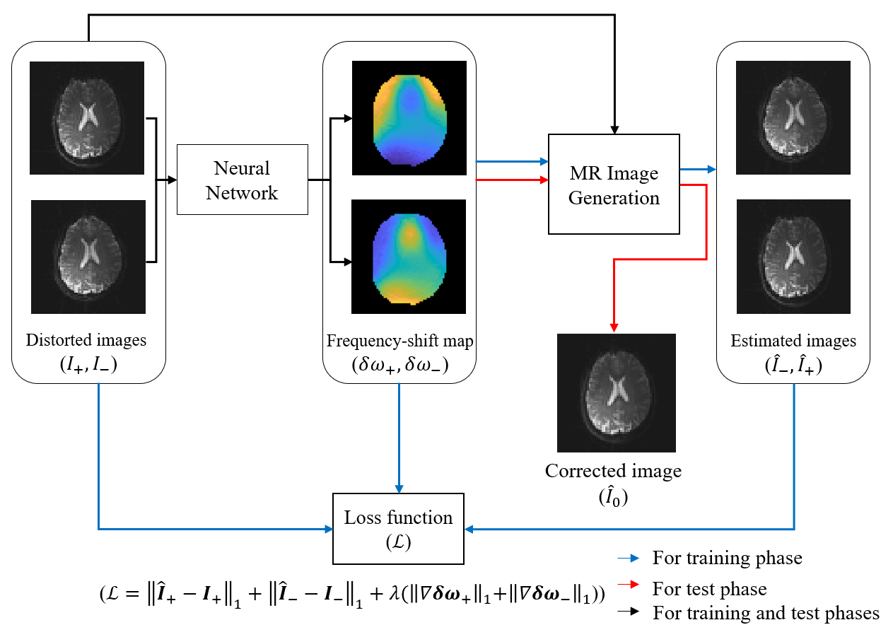
As shown in Fig.1, a correction method of distorted EPI image is proposed, which is an unsupervised learning consisting of a neural network and an MR image generation function. First, the input data of the neural network are distorted images obtained using dual-polarity phase-encoding gradients. By utilizing the MR image generation function, the outputs of the neural network are trained to manifest frequency-shift maps ($$$\delta \omega_+,\ \ \delta \omega_-$$$). Second, the output of the MR image generation function $$$(F_{G_y^{eff}})$$$ represents the reconstructed MR image ($$$\widetilde{I}$$$) acquired with single-shot EPI sequence in the presence of off-resonance frequencies, $$$\delta v=\frac{\gamma}{2\pi}\delta B_0$$$, as follows,
$$\widetilde{I}\left(\widetilde{y}\right)=F_{G_y^{eff}}\left(I,\ \delta v\left(y\right)\right)=\int{\left(\int{I\left(y\right)e^{-j2\pi k_y\left(y+\frac{2\pi\delta v\left(y\right)}{\gamma G_y^{eff}}\right)}dy}\right)e^{j2\pi\widetilde{y}k_y}dk_y}\hspace{0.5cm}(1),$$
where $$$G_y^{eff}=\frac{{\bar{G}}_b\tau}{\mathrm{\Delta}t_y}$$$ is the effective phase-encoding gradients^4-5, and only y direction corresponding to the phase-encoding direction is considered. $$${\bar{G}}_b$$$ is the average blip gradient in the y direction during $$$\tau$$$, $$$\mathrm{\Delta}t_y$$$ is the echo spacing time, $$$y$$$ represents the image domain in the phase-encoding direction, and $$$k_y$$$ represents the corresponding frequency domain. $$$I\left(y\right)$$$ denotes the average proton density at $$$y$$$ including $$$T_1$$$ and $$$T_2$$$ effects. $$$\gamma$$$ is the gyromagnetic ratio of the imaged nuclei. By using the MR image generation function, we can represent frequency-shift maps ($$$\delta \omega_+,\ \ \delta \omega_-$$$) between two distorted images ($$$I_+,\ \ I_-$$$) as follows:
$$\delta \omega_+\left(y^{\prime}\right)=\underset{\delta v}{\operatorname{argmin}}\left \| F_{G_y^{eff}}(I_+\left(y^{\prime}\right),\delta v\left(y^{\prime}\right))-I_-\left(y^{\prime}\right) \right \|_1\hspace{0.5cm}(2),$$
$$\delta \omega_-\left(y^{\prime\prime}\right)=\underset{\delta v}{\operatorname{argmin}}\left \| F_{G_y^{eff}}(I_-\left(y^{\prime\prime}\right),\delta v\left(y^{\prime\prime}\right))-I_-\left(y^{\prime\prime}\right) \right \|_1\hspace{0.5cm}(3).$$
According to Eqs.(2) and (3), by minimizing the input distorted images ($$$I_+,\ \ I_-$$$) and the estimated distorted images ($$${\hat{I}}_+=F_{G_y^{eff}}\left(I_+\left(y^\prime\right),\ \delta \omega_+\left(y^\prime\right)\right)$$$,$$${\hat{I}}_-=F_{G_y^{eff}}\left(I_-\left(y^{\prime\prime}\right),\ \delta \omega_-\left(y^{\prime\prime}\right)\right)$$$), the neural network outputs the frequency-shift maps (blue and black arrows in Fig.1). In order to acquire the smoothed frequency-shift maps the loss function ($$$\mathcal{L}$$$) is defined as follows:
$$\mathcal{L}\left(I_+,I_-\right)=\left \|\hat{I_+}-I_+ \right \|_1+\left \|\hat{I_-}-I_- \right \|_1+\lambda(\left \|\nabla \delta \omega_+ \right \|_1+\left \|\nabla \delta \omega_- \right \|_1)\hspace{0.5cm}(4),$$
where the regularization parameter $$$\lambda$$$ is 0.01 and $$$\nabla$$$ is the spatial gradient operator.
In the test phase (red and black arrows in Fig.1), the distortion-corrected image ($$$\hat{I}_0$$$) is obtained with half of the values of estimated frequency-shift maps ($$$\delta\ \omega_+/2,\ \ \delta\ \omega_-/2$$$) and the two distorted images as follows:
$${\hat{I}}_0\cong\frac{1}{2}\left[F_{G_y^{eff}}\left(I_+\left(y^\prime\right),\frac{1}{2}\delta w_+\left(y^\prime\right)\right)+F_{G_y^{eff}}\left(I_-\left(y^{\prime\prime}\right),\frac{1}{2}\delta w_-\left(y^{\prime\prime}\right)\right)\right]=\frac{1}{2}({\hat{I}}_{+\rightarrow0}+{\hat{I}}_{-\rightarrow0})\hspace{0.5cm}(5).$$
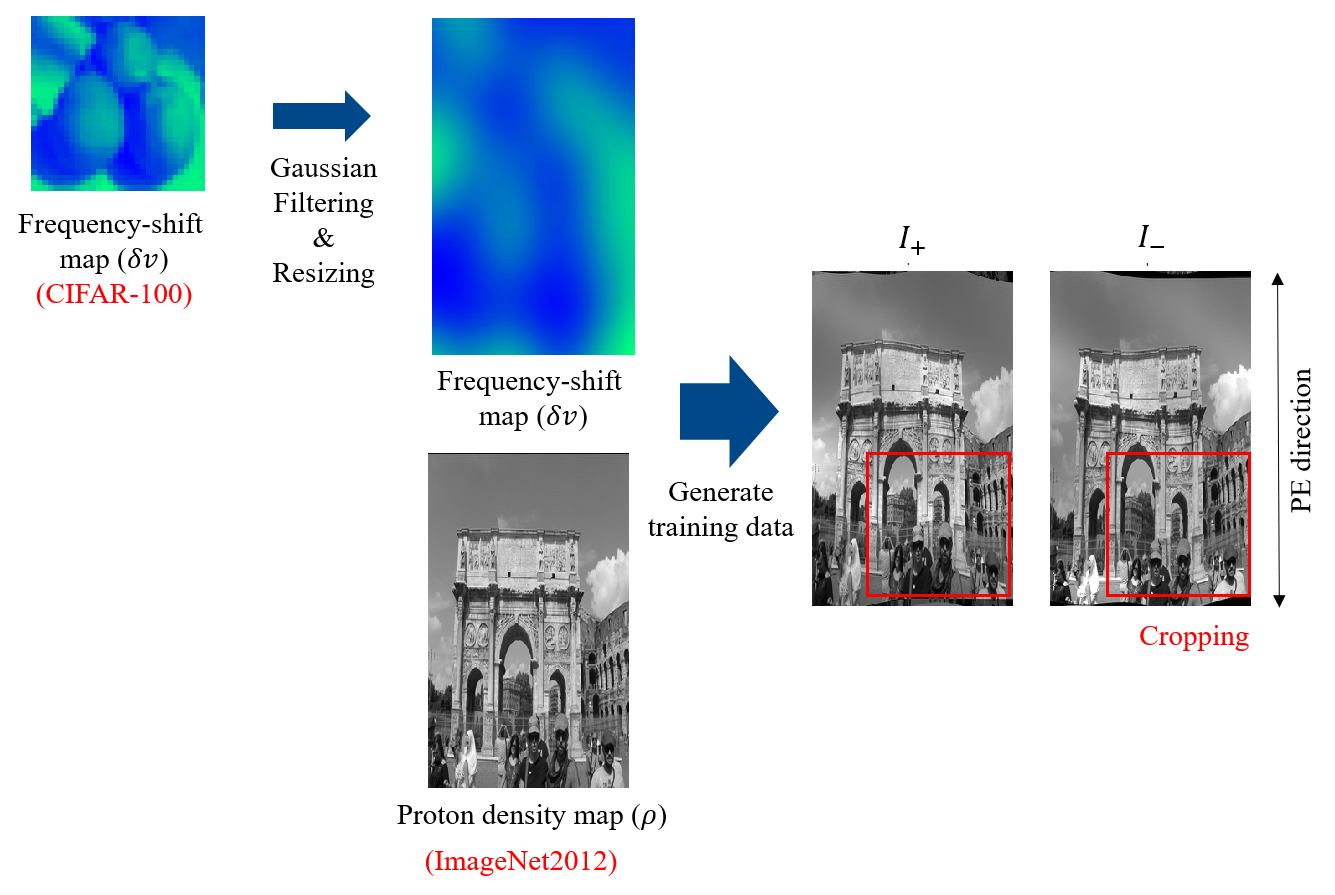
We generated the training datasets with readily available image datasets, such as ImageNet2012⁶ and CIFAR-100, by using MATLAB (Fig.3). The ImageNet2012 datasets represent proton density maps and the Gaussian filtered CIFAR-100 datasets represent frequency-shift maps. The ranges of the frequency-shift maps were set to $$$\pm$$$50Hz. The training datasets were randomly cropped into a size of 64x64 for augmentation and minmax normalization was used.
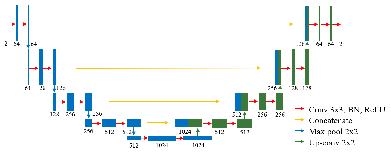
For the neural network, modified U-net⁸ was used in which the ADAM optimizer⁹ with a learning rate of $$${10}^{-4} $$$ was used (Fig.2). 5000 training datasets with a learning batch size of 10 was used.

Results and Discussion

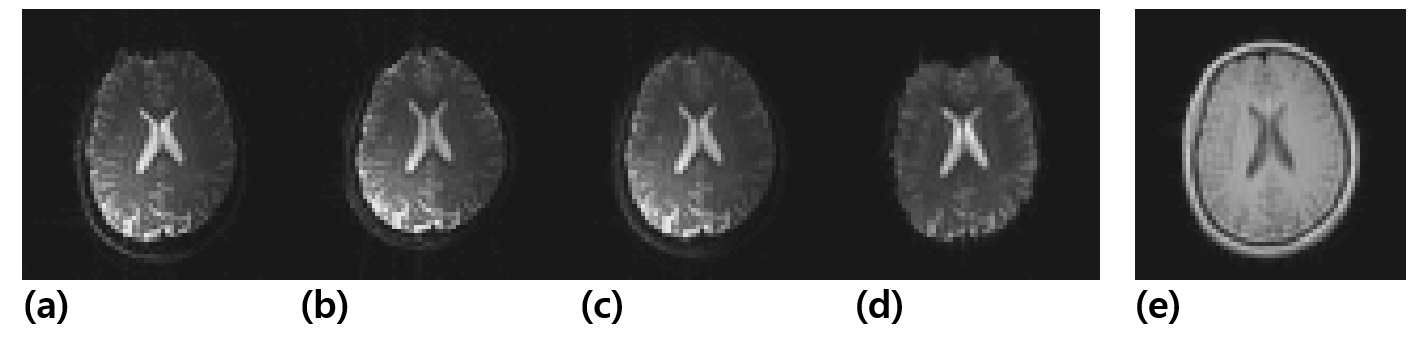
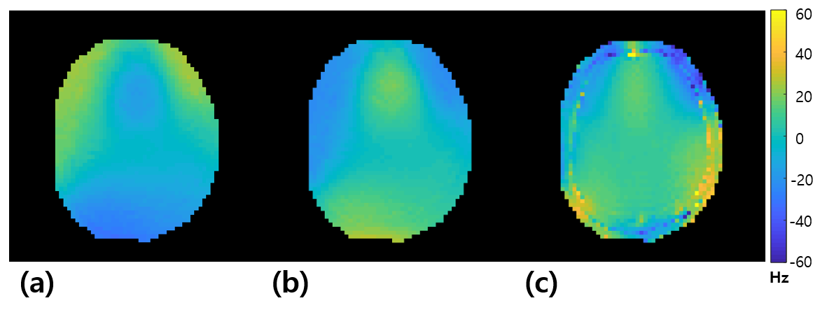
Fig.4 shows that the distortion-corrected image is more structurally similar to the FLASH image compared to the conventional EPI image. Due to B₀ field inhomogeneity, $$$I_+$$$ has distortion at the posterior and $$$I_-$$$ has distortion at the anterior of the brain. The proposed method effectively produced a distortion-corrected brain image. Fig.5 shows the frequency-shift maps in the test phase. The input in-vivo brain image is distorted by the B₀ field inhomogeneity ($$$\delta v$$$) when the image is acquired with an EPI sequence. Because the network outputs the frequency-shift maps ($$$\delta \omega_+,\ \ \delta \omega_-$$$) that maps from $$$I_+$$$ to $$$I_-$$$ or $$$I_-$$$ to $$$I_+$$$, the frequency-shift maps should be twice as large as $$$\delta v$$$. As shown in Fig.5, when half of the network output values are taken, the pattern is similar to the $$$\delta v$$$ or the polarity is reversed; so the network estimates the frequency-shift maps well. Even though the network was trained with synthesized images, the proposed network obtained high-quality distortion-corrected images from real EPI images.

Conclusion

We proposed an unsupervised EPI distortion correction network in the absence of MRI datasets in the training phase. We acquired training datasets by MATLAB simulation of readily available images such as ImageNet2012 and CIFAR-100 datasets which represent proton density maps and frequency-shift maps, respectively. With the MR image generation function, the network was trained to output frequency-shift maps. In the test phase, although the network has not been trained with MRI data, it successfully outputs distortion-corrected EPI images. Also, the proposed method does not need additional frequency-shift map scans for distortion correction.

Acknowledgements

This research was supported by a grant of the Korea Health Technology R&D Project through the Korea Health Industry Development Institute (funded by the Ministry of Health Welfare, Republic of Korea grant number HI 14 C 1135)