Introduction

It is well-known that macroscopic B0 magnetic field inhomogeneities adversely affect quantitative measurements of relaxation parameters obtained with multi-Gradient-Recalled-Echo (mGRE) MRI ^1-4 if not accounted for. It was demonstrated recently that a voxel spread function (VSF) method of correcting field inhomogeneities ⁴ incorporated in a quantitative mGRE-based ⁵ approach provides quantitative information on brain tissue cellular structure ⁶ and its alterations under healthy aging ⁷, and different neurological diseases ^8-11. VSF method takes advantage of utilizing both magnitude and phase of mGRE data from a single scan, hence it saves acquisition time and avoids misregistration errors. In this study, we propose a library-driven approach for VSF calculation that significantly decreases computation time as compared with direct calculation. We also show that image contrasts are improved by incorporating signal decay in VSF calculation.

Methods

As described previously ⁴, the signal of mGRE-MRI can be expressed as: $$S_{n}\left(TE\right)=\sum_m\psi_{nm}\left(TE\right)\cdot\sigma_m\left(TE\right)\space\space\space\space\space\space\space\space\space\space\space\space\space\space\space\space\space\space\space\space\space\space\space\space\space\space\space\space\space\space\space\space\space\space\space\space\space\space\space\space\space\space\space\space\space\space\space\space\left(1\right)$$where $$$S_{n}\left(TE\right)$$$ is the complex image, $$$\sigma_m\left(TE\right)$$$ is the “ideal” signal from the mth voxel. $$$\psi_{nm}\left(TE\right)$$$ is a voxel-dependent convolution kernel, which in 3D case:$$\psi_{nm}\left(TE\right)=\exp\left(i\omega_m\cdot TE+i\phi_0\right)\cdot\eta_x\cdot\eta_y\cdot\eta_z\space\space\space\space\space\space\space\space\space\space\space\space\space\space\space\space\space\space\space\space\space\space\space\space\space\space\space\space\space\space\space\left(2\right)$$where voxel indices n and m are considered as 3D vectors: $$$\left(n_x, n_y,n_z\right)$$$ and $$$\left(m_x, m_y,m_z\right)$$$, $$$\omega_m$$$ represents the frequency shifts. $$$\phi_0$$$ is the signal phase at TE=0. The function $$$\eta$$$ for each dimension is:$$\eta=\sum_qsinc\left(q-q_m\left(TE\right)\right)\cdot\exp\left(2\pi iq\left(n-m\right)\right)\space\space\space\space\space\space\space\space\space\space\space\space\space\space\space\space\space\space\space\space\space\space\space\space\space\space\space\space\left(3\right)$$where q is the 1D normalized k-space defined in the range [-0.5, 0.5]. Parameter $$$q_m$$$ represents the phase dispersion across a voxel:$$q_m\left(TE\right)=\frac{1}{2\pi}\left(g_m\cdot TE+G_m\right)\space\space\space\space\space\space\space\space\space\space\space\space\space\space\space\space\space\space\space\space\space\space\space\space\space\space\space\space\space\space\space\space\space\space\space\space\space\space\space\space\space\space\space\space\space\space\space\space\space\space\space\space\space\space\space\left(4\right)$$where $$$g_m\left(j\right)=\frac{1}{2}\left[\omega_m\left(j+1\right)-\omega_m\left(j-1\right)\right]$$$ and $$$G_m\left(j\right)=\frac{1}{2}\left[\phi_{0m}\left(j+1\right)-\phi_{0m}\left(j-1\right)\right]$$$ are the gradients for the j^th voxel calculated from the spatially unwrapped $$$\omega$$$ and $$$\phi_0$$$, respectively. To solve Eq. (1), similarity approximation was introduced previously ⁴:$$\sigma_m\left(TE\right)\Rightarrow\sigma_n\left(TE\right)\frac{|S_m\left(0\right)|}{|S_n\left(0\right)|}\space\space\space\space\space\space\space\space\space\space\space\space\space\space\space\space\space\space\space\space\space\space\space\space\space\space\space\space\space\space\space\space\space\space\space\space\space\space\space\space\space\space\space\space\space\space\space\space\space\space\space\space\space\space\space\space\space\space\left(5\right)$$In this case, Eq. (1) becomes:$$S_n\left(TE\right)=\sigma_n\left(TE\right)\cdot F_n\left(TE\right)\space\space\space\space\space\space\space\space\space\space\space\space\space\space\space\space\space\space\space\space\space\space\space\space\space\space\space\space\space\space\space\space\space\space\space\space\space\space\space\space\space\space\space\space\space\space\space\space\space\space\space\space\space\space\space\space\space\space\left(6\right)$$and the F-function, which describes the influence of B0 field inhomogeneity on the image:$$F_n\left(TE\right)=\frac{1}{S_n\left(0\right)}\sum_m{\psi_{nm}\left(TE\right)\cdot |S_m\left(0\right)|}\space\space\space\space\space\space\space\space\space\space\space\space\space\space\space\space\space\space\space\space\space\space\space\space\space\space\space\space\space\space\space\space\space\space\space\space\space\left(7\right)$$Since the summation in Eq. (7) extends over many neighboring voxels ⁴, the direct calculation of the F-function for all the imaging voxels requires significant computation time. Herein we propose to use a pre-calculated library for function η in Eq. (3) that is subsequently used in Eq. (7).We also propose to further improve a similarity approximation in Eq. (5) by incorporating into it the signal decay rate R2*:$$\sigma_m\left(TE\right)\Rightarrow\sigma_n\left(TE\right)\frac{|S_m\left(0\right)|\cdot\exp\left(-R2_m^*\cdot TE\right)}{|S_n\left(0\right)|\cdot\exp\left(-R2_n^*\cdot TE\right)}\space\space\space\space\space\space\space\space\space\space\space\space\space\space\space\space\space\space\space\space\space\space\space\space\space\space\left(8\right)$$The main steps of our approach are the following:
(1) Calculation of the 1st-run F-function (F1) using Eq. (5).
(2) Mono-exponential fitting of the complex signal taking into account the function F1 to get $$$|S\left(0\right)|$$$ and the relaxation rate constant R2*.
(3) Calculation of the 2nd-run F-function (F2) using Eq. (8).
All studies were approved by the local IRB. Images were collected from one healthy volunteer (25 years old, male) using a 3T MRI scanner (GE Discovery 750w) equipped with a 12-channel phased-array head coil. High resolution datasets with a voxel size of 1×1×2 mm³ were acquired using a 3D mGRE sequence (ESWAN on GE scanners) with a flip angle of 20° and TR = 53.2 ms. For each acquisition, 10 echoes were collected with first echo time TE1 = 3.3 ms and echo spacing ΔTE = 3.3 ms. The total acquisition time was around 11 min. Complex images from different channels were combined using a previously introduced method ¹². The combined mGRE datasets were then used for calculation of the VSF and R2*. All computations were done in Matlab (2019a, The MathWorks, Inc.) on a computer with standard configurations: 3.2 GHz CPU and 16 GB RAM.

Results

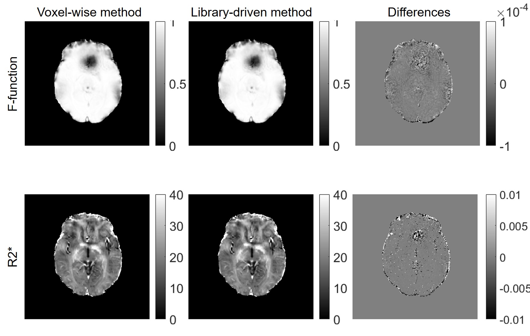
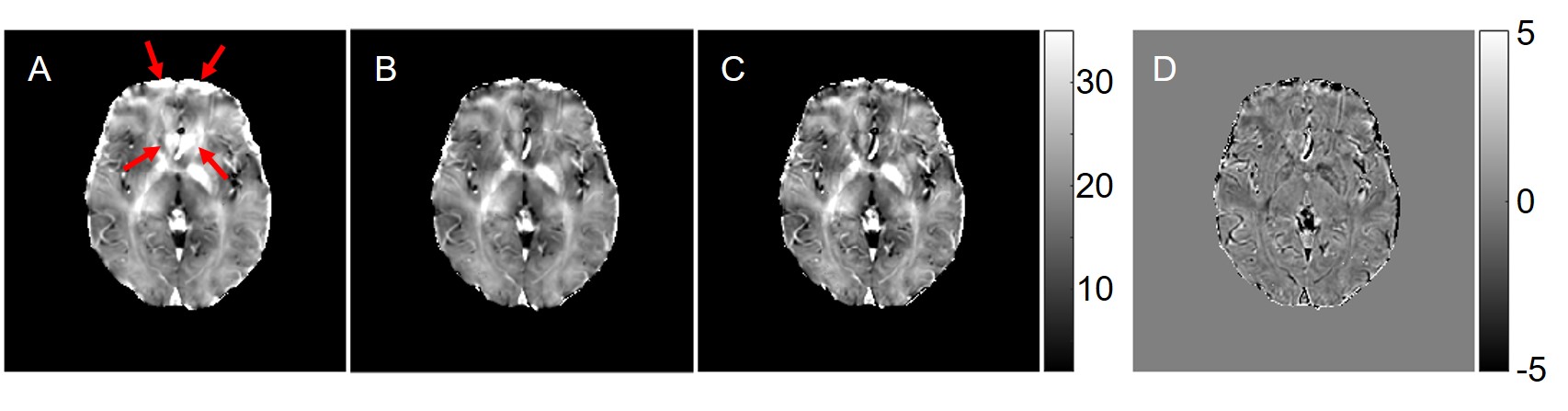
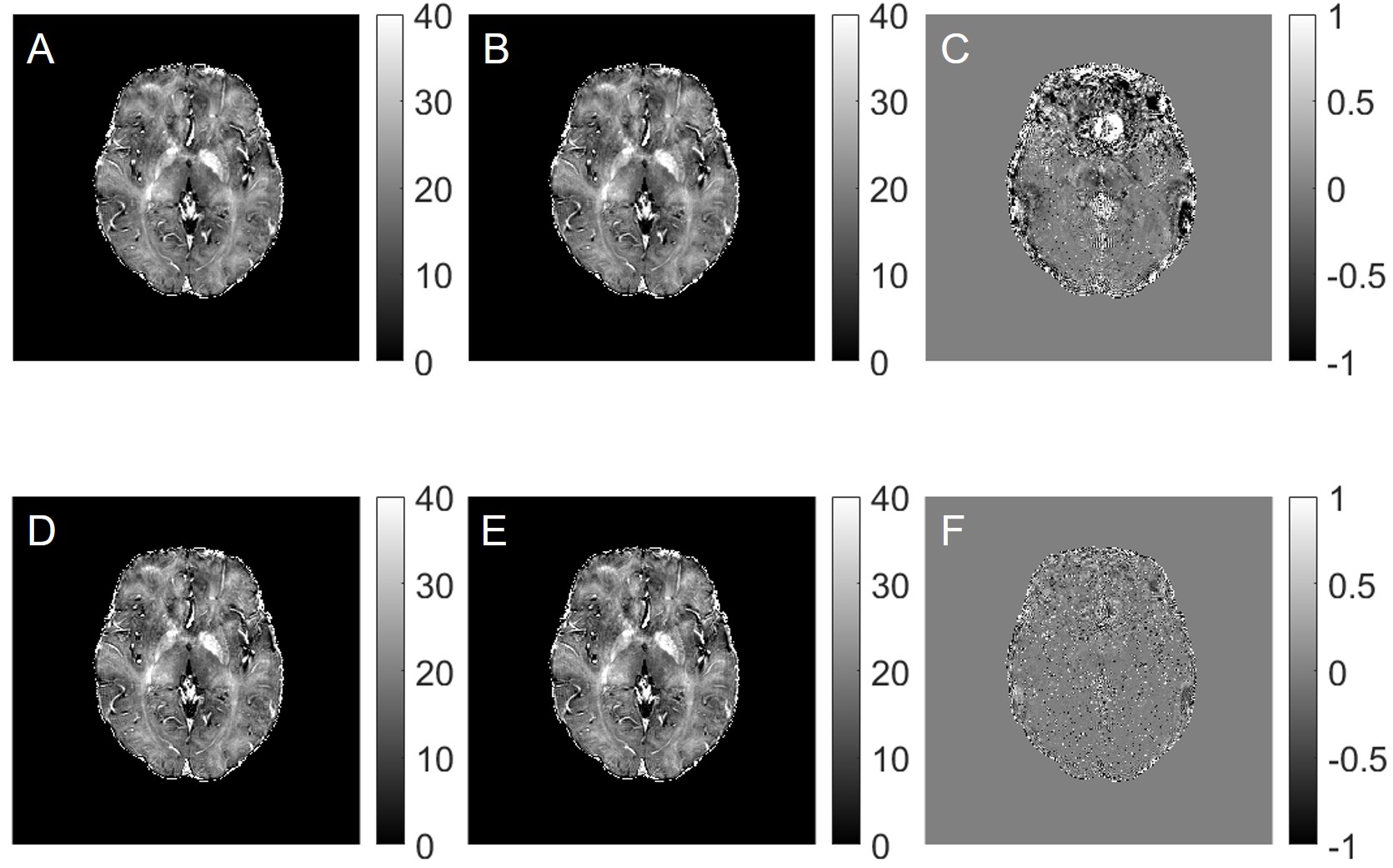
Comparisons of F-functions calculated using direct and new procedure are shown in Fig 1. The direct calculations of F1 and F2 require 5 hours 20 minutes while the new method requires only 3 minutes. Fig 2 shows the comparisons of fitted R2* maps using no F-funtion, F1 and F2. It clearly shows that F-function helped with reducing artifacts on R2* maps, as indicated by red arrows in Fig 2. By using a two-step procedure, the sharpness of R2* is visually enhanced. Fig 3 compares R2* maps calculated using F-functions with different neighbors (4 and 16 neighbors). When F1 was used, the differences between R2* maps are relatively large. When F2 was used, the differences were substantially reduced.

Discussion

Quantitative parameters that are evaluated using mGRE-based techniques are usually affected by magnetic field inhomogeneity effects. These effects cause bias and often corrupt the quantitative measurements, thus hinder the clinical application of these techniques. A VSF method ⁴ allows correction for these effects. In this study, we presented a library-driven approach for fast VSF calculation. By using a pre-calculated library, the F-function calculation time has been reduced from hours (when direct calculation is used) to a few minutes. Additionally, we also incorporated a two-step iterative procedure for VSF calculation that increases the contrast (sharpness) of R2* maps. Our results also showed that by using two-step iterative procedure, the influence of number of neighboring voxels used in calculating F-function for non-hanning filtered data becomes less important (Fig 3). One can always use 4 neighbors to calculate F-function, which helps to further reduce computing time when non-hanning filtered datasets are used.

Conclusion

We presented a library-driven approach for fast two-step iterative VSF calculation. The new procedure provides a fast way to correct for background field inhomogeneity artifacts, thus can facilitate the applications of mGRE-based quantitative techniques in clinical practices.

Acknowledgements

This work was supported by “the Fundamental Research Funds for the Central Universities” and “the Research Start-up Funds” from the First Affiliated Hospital of USTC.