Introduction

Single-shot acquisitions allow for high temporal resolution and are robust against motion making them the method of choice for several applications such as fMRI, DWI or ASL. However, a main limiting factor are artifacts introduced due to B₀ inhomogeneities, in particular when aiming for high resolution. The related artefacts can be addressed in the image reconstruction when incorporating knowledge of the B₀ distribution, which is commonly provided by a field map obtained by separate multi-echo GRE imaging¹. However, calculating accurate B₀ maps requires multiple post-processing steps (like masking), which are prone to errors. In addition, the acquisition takes time, and inter-scan motion can render the maps invalid. For these reasons, B₀ off-resonance is often neglected in practice. To address these issues, algorithms have been devised to correct the acquired data without the need of a preparation scan^2,3 requiring specific k-space trajectories. A generic approach is to jointly estimate B₀ map and object by minimizing signal model violations³. Yet, this method is not widely used, presumably owing to the choice of the algorithm to handle the involved non-convex optimization problem. In this work, a novel algorithm is proposed that improves convergence to meaningful solutions of this non-convex optimization problem, i.e. estimating B₀ and reconstructing the object. First imaging results are presented using standard single-shot EPI and Spiral sampling (R=3). Moreover, the correction of motion induced B₀ artefacts is shown as an application.

Methods

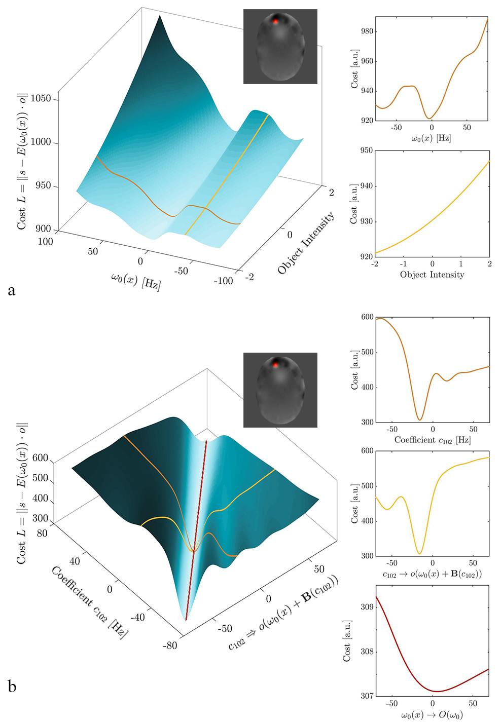
A Cost Function in B₀
Given the acquired signal $$$s(t)$$$, the object $$$o(\textbf{x})$$$ and the field map $$$\omega_0(\textbf{x})$$$ can be obtained by minimizing the cost function $$$L$$$

$$L(\omega_0(\textbf{x}),o(\textbf{x}))=\Vert\,s(t)-E(\textbf{k}(t),\omega_0(\textbf{x}))\cdot o(\textbf{x})\Vert^2\rightarrow\text{min}\;\;\;(1)$$
with the encoding matrix $$$\textbf{E}$$$ having entries
$$E_{mn}=\exp(-i\omega_0(\textbf{x}_n)t_m)\cdot\exp(-i2\pi\textbf{k}(t_m)\cdot\textbf{x}_n).$$
The cost is convex in $$$o(\textbf{x})$$$ and non-convex in $$$\omega_0(\textbf{x})$$$ as depicted in Figure 1a.
It was proposed previously to solve the problem by alternating the following two steps²:

(i) Reconstructing an object $$$o_i(\textbf{x})$$$ for the current B₀ map guess $$$\omega_{0,i}(\textbf{x})$$$
(ii) Optimizing$$$\;\omega_{0,i}(\textbf{x})\rightarrow\omega_{0,i+1}(\textbf{x})\;$$$while fixing $$$o_i(\textbf{x})$$$.

Alternating optimization converges in general quickly only for loosely coupled variables⁴. However, the variables are strongly coupled by an image reconstruction accounting for B₀^5,6
$$o(\textbf{x})=\left(E^H(\textbf{k}(t),\omega_0(\textbf{x}))\,E(\textbf{k}(t),\omega_0(\textbf{x}))\right)^{-1}\,E^H(\textbf{k}(t),\omega_0(\textbf{x}))\cdot\,s(t)\;\;\;(2)$$
which can be exploited by inserting (2) into (1) leading to
$$L(\omega_0(\textbf{x}))=\Vert\sigma(\textbf{k})\cdot(s(t)-\left(E^H(\textbf{k},\omega_0)\,E(\textbf{k},\omega_0)\right)^{-1}\,E^H(\textbf{k},\omega_0)\cdot\,s(t))\Vert^2\rightarrow\text{min}.\;\;\;(3)$$
Here, $$$\sigma(\textbf{k})$$$ denotes a k-space filter to reduce the strong weighting of signal from the k-space center. The resulting search space is rearranged such that objects reconstructed with similar field maps and hence similar distortions are close to each other in a Euclidean sense but still exhibits a non-convex structure (Figure 1b). However, the resulting cost is only a function in $$$\omega_0(\textbf{x})$$$ which reduces the dimensionality of the search space drastically and searching for a minimum means traversing along the tuples $$$(\omega_0(\textbf{x}),o(\omega(\textbf{x})))$$$ allowing for greater step sizes (red line Figure 1).
Note that a reconstructed object is obtained as an intermediate result when evaluating the cost $$$L$$$ as described in equation (3).

Optimization Strategy and Regularization
Since the bulk information of the B₀ distribution can be represented on a coarser resolution^7,8, a smoothness constraint on B₀ may be applied to stabilize convergence and speed-up the algorithm⁹. This is implemented by approximating B₀ by a sum of Gaussians ($$$\sigma=0.8$$$) weighted by coefficients $$$c_i$$$ on a grid with grid points $$$x_i$$$:
$$\omega_0(\textbf{x})\approx\,B(c_i):=\sum_i\,c_i\cdot\beta(x-x_i).$$
In the current implementation, the dimensionality of the problem can thereby be reduced from ~50’000 (#voxels) to around 400 (20x20 coefficients). To minimize $$$L$$$, a standard gradient descent with discrete gradient calculations is performed to update the coefficients of the vector$$$\;c_i$$$:
$$c_{i+1,j}=c_{i,j}+\frac{L(B(c_i+\Delta\omega\cdot\,e_j))-L(B(c_i))}{\Delta\omega}$$
with a unit vector$$$\;e_j\;$$$and$$$\;\Delta\omega=0.2\text{Hz}$$$. To further decrease the number of local minima, $$$\sigma(\textbf{k})$$$ is set to mask the resolution of the used data to the B₀ map's target resolution.

MR Experiments
Measurements were performed on a 3T MR system (Philips Healthcare, Best, The Netherlands) using a 16-channel head coil with integrated magnetic field sensors¹⁰ (Skope MR Technologies, Zurich, Switzerland) to record the actual k-space trajectory. EPI and Spiral scans were played out with a TE of 24ms (FOV=22cm, in-plane resolution 1mm, R=3). As a reference, a field map from a 4-echo GE sequence $$$(\Delta t=1.2\text{ms})$$$ was fitted. To investigate motion related effects on B₀, a subject was instructed to nod and remain in the position for a second scan.

Results

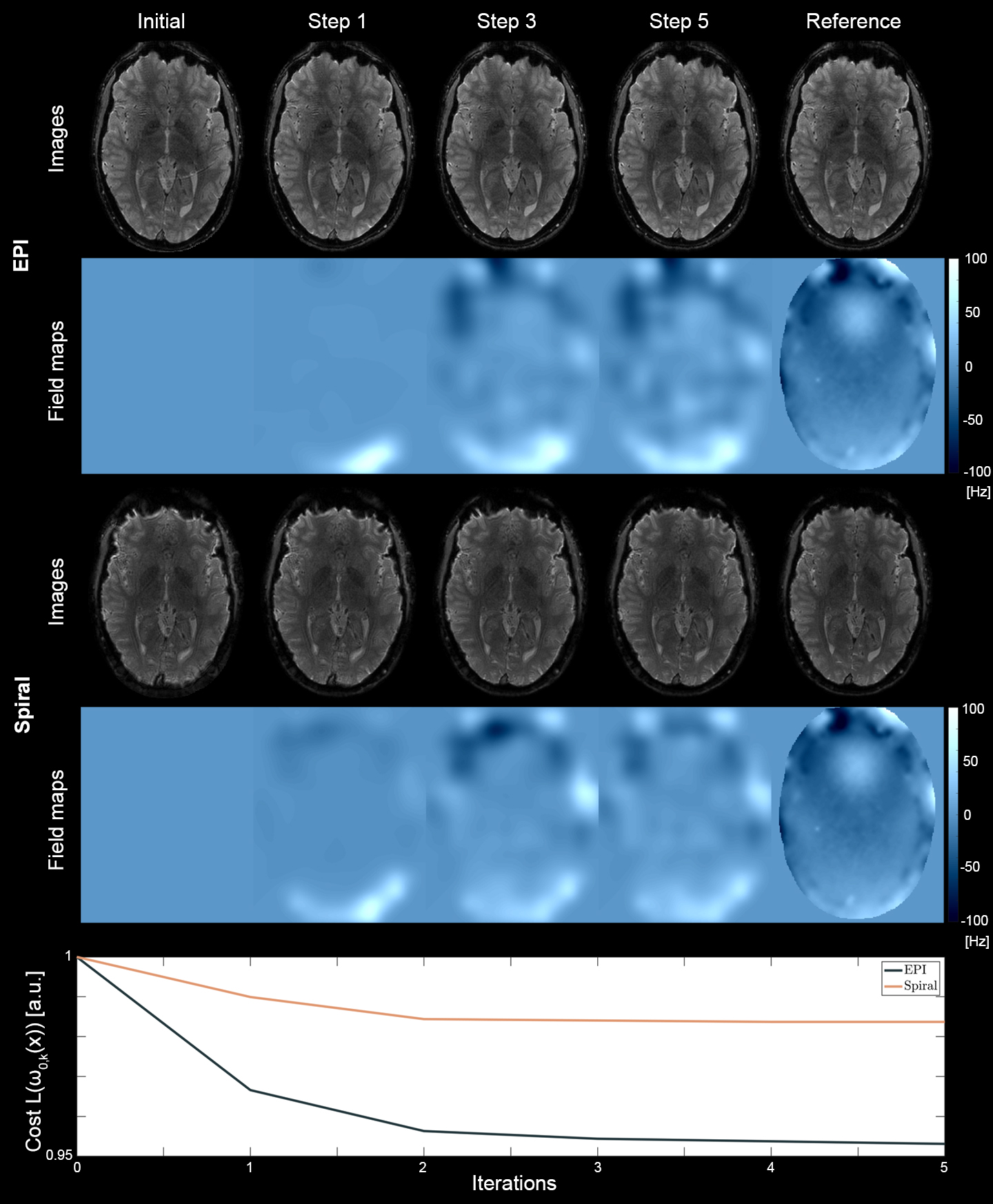
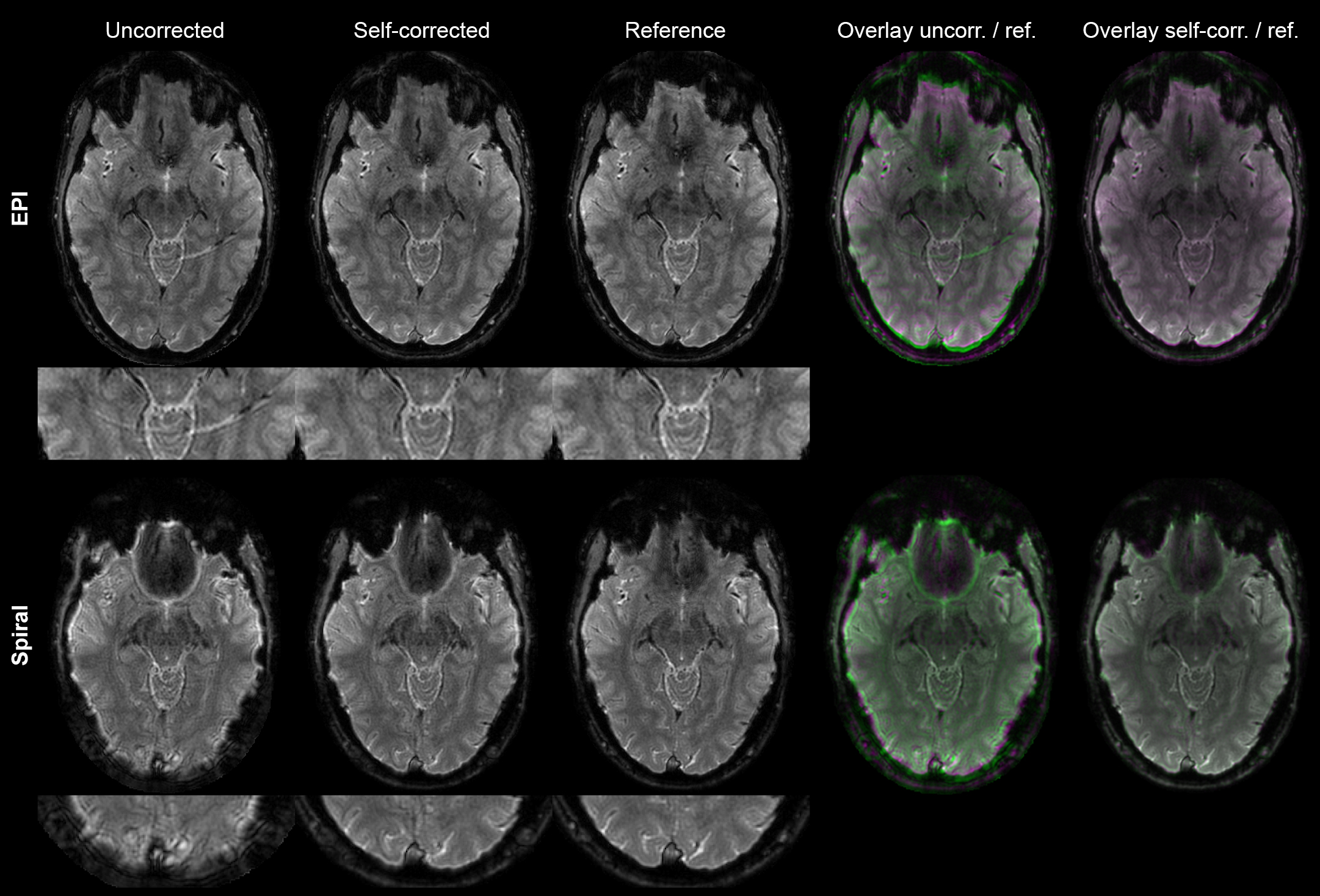
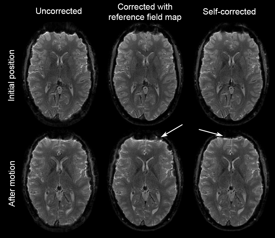
The field maps found by the proposed method converged towards the measured gradient echo field map; at the same time the cost is reduced in each iteration step until convergence (Figure 2). Also in lower slices the algorithm was capable of reducing B₀ related artifacts i.e. blurring in Spiral and local image shifts and related ghosting in EPI readouts (Figure 3). The method also proved useful to correct for motion induced B₀ changes, which cannot be accounted for when employing pre-acquired B₀ maps (Figure 4).

Discussion and Conclusion

The method significantly improved image quality for all tested cases, indicating that the proposed cost function and regularization is capable of solving the non-convex B₀ estimation problem. Single-shot EPI and Spirals (R=3) without explicit k-t sampling were used as readouts, indicating that the multi-channel array implicitly encodes B₀ information by requiring consistency among the sampled k-t space.

Acknowledgements

No acknowledgement found.