3394
Comparison of three B1 correction methods for RARE imaging with transceive surface RF coils
Paula Ramos Delgado1, Andre Kuehne2, Jason M. Millward1, Joao Periquito1, Thoralf Niendorf1,3, Sonia Waiczies1, and Andreas Pohlmann1
1Berlin Ultrahigh Field Facility (B.U.F.F), Max Delbrück Center for Molecular Medicine in the Helmholtz Association, Berlin, Germany, 2MRI.tools GmbH, Berlin, Germany, 3Experimental and Clinical Research Center, a joint cooperation between the Charité Medical Faculty and the Max Delbrück Center for Molecular Medicine in the Helmholtz Association, Berlin, Germany
1Berlin Ultrahigh Field Facility (B.U.F.F), Max Delbrück Center for Molecular Medicine in the Helmholtz Association, Berlin, Germany, 2MRI.tools GmbH, Berlin, Germany, 3Experimental and Clinical Research Center, a joint cooperation between the Charité Medical Faculty and the Max Delbrück Center for Molecular Medicine in the Helmholtz Association, Berlin, Germany
Synopsis
Fluorine MR methods support quantification but have inherently low SNR. To enhance sensitivity, SNR-efficient imaging techniques such as RARE and cryogenically-cooled surface RF coils are used. However, transceive surface RF coils show variation in the excitation field, impairing quantification and T1 contrast. We previously showed improved homogeneity using a novel B1 correction method developed for 1H imaging that uses experimental data acquired with a volume resonator. Here, we compared it to a sensitivity-only correction and a combination of both, to evaluate which approach yields the most accurate contrast and concentration quantification. This work is applicable to different nuclei.
Introduction
Fluorine (19F) MRI methods have demonstrated promising results for the non-invasive monitoring of exogenous fluorinated labels in vivo1-8. Given the lack of organic 19F in living tissues, the obtained signal is highly specific and supports quantification, but it is severely reduced due to the low signal-to-noise ratio (SNR) provided by the acquisition methods9-10. A way to overcome the sensitivity limitations is to use a combination of SNR-efficient imaging techniques such as RARE11 and state-of-the-art cryogenically-cooled probes (CRP)12. However, CRPs are only available as transceive surface coils and thus show substantial variation in the excitation (B1+) and sensitivity (B1-) fields12-14. This characteristic makes them impractical for achieving meaningful quantification and tissue contrast. Previous research has focused on retrospective B1+ correction methods which use analytical equations that describe the relationship of signal intensity (SI) and flip angle (FA) of particular MRI sequences. While this approach has been successfully applied to gradient echo techniques like FLASH15-16, it is not feasible for RARE due to its more complex train of spin-echoes and stimulated echoes for which no analytical SI equation exists17-18. Previously we demonstrated the efficacy of a novel method developed for 1H imaging to correct B1 inhomogeneities in transceive surface RF coils with RARE using a numerical model which described SI as a function of the FA and T119. Here, we evaluate performance of this method compared to a sensitivity-only correction method and a hybrid combination of both, to determine which approach yields the most accurate contrast and concentration quantification. This work is applicable to different nuclei.Methods
Sample preparation and MR measurementsFour phantoms (50ml flasks) were prepared with two different 1H-atom concentrations (100% water, 50%-50% water/deuterium oxide) and two different T1 (490ms, 1525ms; achieved via added gadolinium-based contrast agent). Experiments were performed on a 9.4T animal MR scanner (Bruker BioSpin, Ettlingen, Germany). RARE images (TE/TR=5.1/1000ms, ETL=8, BW=50kHz, centric encoding, resolution=(273x273)mm2, 3 axial slices of 2mm thickness with 0.5mm gap, 30min) were acquired using a 1H transceive surface loop RF coil. Reference power adjustments were performed on a 2mm slice parallel to the RF coil surface. Reference images and T1 maps (RARE: 8 TRs, 200-9000ms) were acquired using a volume resonator.
Correction methods
Fig.1 shows a summary of the three processing pipelines:
Model-based B1 correction: A phantom with a short T1 of 280ms was utilized to compute a B1+ map using the double angle method20-21 and a B1- map using the low FA approximation22-23. A SI model was calculated from RARE scans (same parameters as above, FA between 5º-110º) of 19 NMR tubes (gadolinium-doped water mixtures, T1: 170–2600ms) using a volume resonator. The corrected images were calculated as described previously19.
Sensitivity correction: A RARE image (same parameters) was acquired using the above phantom and its SI normalized. The sensitivity of each of the remaining phantom images was corrected multiplying by the inverse of this normalized image.
Hybrid B1 correction: B1+ correction was performed using the model-based approach, followed by B1- correction using the sensitivity correction method.
Performance assessment
Concentration quantification: the proportionality of the SI to the number of atoms was evaluated using pairs of phantoms with different water content and the same T1 value (Fig.2). Six random ROIs were drawn (Fig. 3C) and applied to the images (Fig. 3) to calculate mean SI ratios ($$$\overline{SI}$$$) for 18 combinations of two ROIs for each image. The error in quantification was computed as $$$\frac{\overline{SI_{reference}}-\overline{SI_{corrected}}}{\overline{SI_{reference}}}\cdot100$$$ (%). Finally, the mean error and mean standard deviation were calculated.
T1 contrast: the same procedure was followed using pairs of phantoms with the same water content and different T1 values.
Results
While uncorrected images showed substantial errors (35-44%) and variabilities in all cases, the correction methods reduced the mean errors to less than 10% for both quantification and contrast (Fig.4-5). Sensitivity correction performed well when calculating water content proportions at low T1 values (4.6±3.5%), closely followed by the hybrid (5.3±3.1%) and model-based (6.4±4.8%) methods. All three methods behaved similarly for higher T1 values, with mean errors of approximately 10%. When measuring T1 contrast, the hybrid method performed best for both water content phantoms (2.4±1.6% high, 4.5±3.9% low). The sensitivity correction method performed better than the model-based method for the high water content phantom (3.1±2.8% vs. 5.7±5.1%). However for the low water content phantom the model-based correction method performed better than the sensitivity correction method (4.7±4% vs. 9.2±2.6%).Conclusions
Here we showed a comparison of two B1+/B1- correction methods (model-based, hybrid) and a simple B1- (sensitivity) correction method. All three methods performed similarly for quantifying concentration, and all performed better for low T1 values compared to high T1 values. One explanation for this is that with low T1 there was effectively less T1-weighting for the used TR, and thus less correction was needed. For preserving T1 contrast, the hybrid correction method performed better than the other two. Therefore, we suggest using a simple sensitivity correction when quantifying the number of atoms (e.g. of 19F-loaded nanoparticles). However, when T1 contrast is essential (e.g. 1H imaging) a hybrid B1 correction provides more accurate results.Acknowledgements
This work was supported by the Deutsche Forschungsgemeinschaft to S.W. (DFG-WA2804) and A.P. (DFG-PO1869).References
- Khalil AA, et al. Longitudinal 19F magnetic resonance imaging of brain oxygenation in a mouse model of vascular cognitive impairment using a cryogenic radiofrequency coil. MAGMA (2019); 32(1): 105-14.
- Waiczies H, et al. Visualizing brain inflammation with a shingled-leg radio-frequency head probe for 19F/1H. Sci Rep (2013); 3: 1280.
- Flögel U, et al. Noninvasive detection of graft rejection by in vivo 19F MRI in the early stage. Am J Transplant (2011); 11(2): 235-44.
- van Heeswijk RB, et al. Fluorine-19 magnetic resonance angiography of the mouse. PloS ONE (2012); 7(7): e42236.
- Bar-Shir A, et al. Single 19F probe for simultaneous detection of multiple metal ions using miCEST MRI. J Am Chem Soc (2015); 137(1): 78-81.
- Moonshi S, et al. A unique 19F MRI agent for the tracking of non phagocytic cell in vivo. Nanoscale (2018); 10: 8226-39.
- Ribot EJ, et al. In vivo MR detection of fluorine-labeled human MSC using the bSSFP sequence. Int J Nanomedicine (2014); 9: 1731-39.
- Bonetto F, et al. A novel 19F agent for detection and quantification of human dendritic cells using magnetic resonance imaging. Int J Cancer (2012); 129(2): 365-73.
- Ruiz-Cabello J, et al. Fluorine (19F) MRS and MRI in biomedicine. NMR Biomed (2011); 24(2):114-129.
- Waiczies S, Ji Y, Niendorf T. Tracking methods for dendritic cells. Fluorine Magnetic Resonance Imaging (2017); chapter 9: 243-281.
- Hennig, J, et al. RARE imaging: a fast imaging method for clinical MR. Magn Reson Med, 1986; 3: 823-833.
- Waiczies S, et al. Enhanced fluorine-19 MRI sensitivity using a cryogenic radiofrequency probe: technical developments and ex vivo demonstration in a mouse model of neuroinflammation. Sci Rep (2017); 7: 9808.
- Axel L, Hayes C. Surface coil magnetic resonance imaging. Archives Internationales de Physiologie et de Biochimie (1985); 93(5): 11-18.
- Baltes C, et al. Micro MRI of the mouse brain using a novel 400 MHz cryogenic quadrature RF probe. NMR Biomed (2009); 22(8): 834-42.
- Wang J, Qiu M, Constable R T. In vivo method for correcting transmit/receive nonuniformities with phased array coils. Magn Reson Med (2005); 53: 666-674.
- Vernikouskaya, I, et al. Quantitative 19F MRI of perfluoro-15-crown-5-ether using uniformity correction of the spin excitation and signal reception. MAGMA (2019); 32(1): 25-36.
- Conturo E, et al. Simplified mathematical description of longitudinal recovery in multiple-echo sequences. Magn Reson Med (1987); 4: 282-88.
- Meara SJP, Barker GJ. Evolution of the longitudinal magnetization for pulse sequences using a fast spin-echo readout: application to fluid-attenuated inversion-recovery and double inversion-recovery sequences. Magn Reson Med (2005); 54: 241-45.
- Ramos Delgado P, et al. Retrospective transmission field (B1+) and sensitivity profile (B1-) correction for transceive surface RF coils: an empirical solution for RARE. Proceedings of ISMRM Montréal 2019, No. 4502.
- Akoka, S, et al. Radiofrequency map of an NMR coil by imaging. Magn Reson Imaging (1993); 11:437-441.
- Insko, EK, et al. Mapping of the radiofrequency field. J Magn Reson (1993); A103:82-85.
- Ibrahim T S, Hue Y-K, Tang L. Understanding and manipulating the RF fields at high field MRI. NMR in Biomed (2009); 22: 927-36.
- Pauly J, Nishimura D, Macovski A. A k-space analysis of small-tip-angle excitation. J Magn Reson (1989); 43-56.
Figures
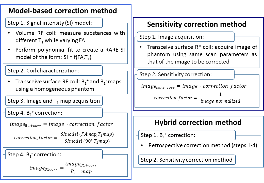
Figure 1. Pipeline description of two compared B1+/B1- correction methods (model-based,
hybrid) and a simple B1- (sensitivity) correction method.
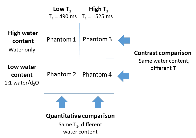
Figure 2. Experimental setup. We used four phantoms
(50 ml flasks) with two different 1H-atom concentrations (100%
water, 50%-50% water/deuterium oxide) to which we added gadolinium in order to achieve
two different T1 relaxation times (490 ms,1525 ms). This
experimental setup allowed quantitative comparisons of the corrected signal
intensity for low and high T1 values and T1 contrast
comparisons for high and low water content.

Figure 3. Illustration of performance
assessment using example figures from one flask (T1=490ms, water
only). (A) original image measured
with the transceive surface RF coil, (B)
reference image acquired with the volume RF coil, (C) ROI placement of 6 randomly-selected locations used for
performance assessment, (D)
model-based-corrected image, (E)
sensitivity-corrected image, (F)
hybrid-corrected image. The position of the 1H transceive surface
loop RF coil is shown with a dashed white line.
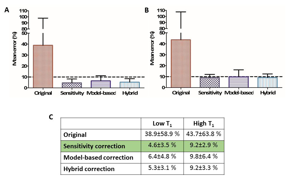
Figure 4. Performance of concentration quantification. (A) Plot of mean errors and
standard deviations for the original image and the three correction methods for
low T1 relaxation times. (B) Plot of mean errors and standard
deviations for the original image and the three correction methods for high T1
relaxation times. (C) The calculated
values; the best performing method is highlighted in green.

Figure 5. T1
contrast performance. (A) Plot of mean errors and standard deviations for the original image and
the three correction methods for high water content. (B) Plot of mean errors
and standard deviations for the original image and the three correction methods
for low water content. (C) The
calculated values; the best performing method is highlighted in green.