Introduction

MRI with spiral trajectory is a fast and efficient scanning strategy that may benefit cardiovascular and functional brain imaging. Its clinical application is however challenged by notorious sensitivity to gradient trajectory deviation from design, resulting from factors including gradient delay, eddy currents, and imperfections in the gradient amplifier. Existing trajectory correction techniques include gradient field measurement, gradient system calibration, and delay correction, among others [1-5].
In this study a new comprehensive spiral gradient waveform correction strategy is proposed that features multipoint gradient anchoring (MGA). By measuring multiple gradient delays in spiral waveforms at different rotation angles, it effectively ‘anchors’ the waveform at a series of known locations. MGA can measure the whole trajectory and improve waveform fidelity by only relying on several additional prescan acquisitions with limited time cost; prior information of the gradient system response is not necessary.

Theory

Clinical spiral imaging typically involves multiple interleaves to cover the entire k-space. Typically, one such basis interleaf is designed first and then rotated by various angles to generate other interleaves. For simplicity only x-axis is discussed below but the approach is generally applicable. Let \({G_{xo}}(t)\) and\({G_{yo}}(t)\) be the x and y gradient waveform of the basis interleaf respectively, then the x gradient waveform of an interleaf rotated by \(\theta \) is:
$${G_x}(\theta ,t) = \cos (\theta )*{G_{x0}}(t) + \sin (\theta )*{G_{y0}}(t) $$
,where t is the readout time and indexed from 1 to m.

Since k-space locations are determined by the time integral of the gradient waveform, if linear system is assumed, the k-space deviation \(\Delta {K_x}(\theta ,t)\) of any interleaf from design trajectory will have a similar relation with that of the basis interleaf:
$$\Delta {K_x}(\theta ,t) = \cos (\theta )*\Delta {K_x}_0(t) + \sin (\theta )*\Delta {K_{y0}}(t) $$

With acquisitions at multiple angles \({\theta _1},{\theta _2}, \ldots ,{\theta _n}\) we have:
$${\rm{Kx}} = {\rm{\Theta x}}*\Psi $$
,where \({\rm{Kx}}\) is a matrix with \({\rm{K}}{{\rm{x}}_{{\rm{i,j}}}}{\rm{ = }}\Delta {K_x}({\theta _i},{t_j})\), i = 1,2,…,n, and j=1,2,…,m. \({\rm{\Theta x}}\) is a rotation matrix of size n by 2, with its ith row being \([\cos (\theta ),\sin (\theta )]\). \(\Psi \) is a matrix of size 2 by m and formed by concatenating \(\Delta {K_x}_0\) and \(\Delta {K_y}_0\).

Building upon a previous approach to measure gradient delay using prescan [Ref 4], k-space shifts can be estimated at every k-space zero-crossing, instead of a same value that fits all. Specifically, by comparing spirals acquired at rotation angles of \({\theta _p}\) and \({\theta _p} + \pi \) when only enabling x-axis gradient, a shift value can be determined whenever their trajectories cross at k-space origin (Fig. 1). Subsequently each shift value is written to fill the matrix at \({\rm{K}}{{\rm{x}}_{{\rm{i,j}}}}\) where \({\theta _i} = {\theta _p}\) and \({t_j}\) is the nearest time at which the crossing occurs when design trajectory is assumed.

The objective of spiral waveform correction is equivalent to knowing \(\Delta {K_x}_0\) and \(\Delta {K_y}_0\) at every readout time. Although theoretically \(\Psi \) can be obtained by solving the above equation, in reality \({\rm{Kx}}\) is sparse with limited number of elements due to limited zero-crossings. However these elements can still serve as ‘anchors’ that fixate \(\Psi \) at multipoints in the proposed MGA technique, largely reducing its degree of freedom. A number of approaches can be further used to recover \(\Psi \), for example by constrained optimization considering the facts that \(\Psi \) should be slowly varying in time and that the echo signal should maintain its shape across various zero-crossings. Here as a proof-of-concept, simple linear interpolation was used for \(\Delta {K_x}_0\) and \(\Delta {K_y}_0\) data points away from the anchors and a simple waveform measurement was performed based on reference [7] but only covers the beginning portion of \(\Psi \).

Methods

A prototype spiral sequence was implemented on a clinical 1.5T scanner (uMR 560, United Imaging Healthcare, Shanghai, China). Spiral imaging with evenly angular distribution were tested on both phantom and human brain. Imaging parameters, including the number of anchors used in prescan, were summarized in Table 1. To demonstrate the proposed MGA technique can work under various conditions, 3 different combinations of typical imaging parameters were used. Reconstruction was done offline using regridding with Kaiser-Bessel kernel, with and without MGA technique.

Results

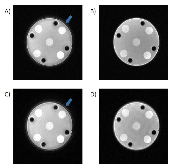
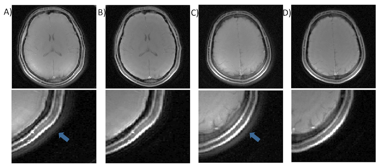
Images acquired and reconstructed with the proposed MGA technique showed little blurring or ringing artifact associated with uncorrected gradient trajectory, under different imaging parameters, while images without correction have obvious artifacts (Fig.2). Typical images of the brain from a healthy volunteer demonstrated consistent good quality across slices with MGA (Fig.3).

Conclusion and Discussions

The proposed MGA technique is an effective and simple method to correct spiral imaging trajectories with minimal time cost. The technique is essentially self-calibration in nature and no prior assumption of the gradient system is needed. It is expected to be less susceptible to system variation and mischaracterization. Although only cases with evenly angular distribution were demonstrated, it is obvious that as long as effective coverage of k-space is achieved as in most imaging scenarios, MGA is expected to work. Extensive testing is currently underway to verify MGA’s application in more applications.

Acknowledgements

No acknowledgement found.