3384
MRI Scanner Characterization with the ISMRM/NIST System Phantom1National Institute of Standards and Technology, Boulder, CO, United States, 2American College of Radiology, Philadelphia, PA, United States, 3Duke Image Analysis Laboratory, Durham, NC, United States, 4Merck Research Laboratories, West Point, PA, United States, 5Mayo Clinic, Rochester, MN, United States, 6University College London, London, United Kingdom, 7University of Wisconsin, Madison, WI, United States, 8National Institute of Biomedical Imaging and Bioengineering, Bethesda, MD, United States, 9University of Washington, Seattle, WA, United States
Synopsis
We describe basic scanner characterization and determination of MR-parameter measurement accuracy using the ISMRM/NIST system phantom. The phantom provides a convenient method to measure geometric distortion; the efficacy of non-linear gradient corrections; slice profiles and associated measurement uncertainties; protocol and system dependent resolution contributions; SNR according to NEMA protocols; accuracy of relaxation time; and proton density measurements. The phantom is unique in having SI-traceability, a high level of precision, long-term stability, and monitoring by a national metrology institute.
Introduction
The ISMRM ad hoc Committee on Standards for Quantitative Magnetic Resonance and NIST, have designed and commercialized a standard MRI system phantom(1) to assess scanner performance, scanner stability, scanner inter-comparability and accuracy of quantitative relaxation time imaging. The phantom is unique in having SI-traceability(2), a high level of precision, long-term stability, and monitoring by a national metrology institute. The system phantom, or modified versions of it, have been used for several studies including repeatability of MR fingerprinting (3), assessing changes occurring during scanner upgrades (4), and assessing variation in multi-site T1 measurements (5). Many other uses are ongoing, including monitoring of scanners for quality assurance and homogenizing scan protocols across multi-vendor scanners. Here, we describe the use of the phantom to measure fundamental MRI parameters including geometric distortion, resolution, slice profile, and proton density. We present standard measurement and analysis protocols. The standard measurement protocols are not meant to be the best measurement methods, rather they are meant to form a common baseline upon which improved protocols can be benchmarked. We show that the phantom provides important information on scanner performance including the accuracy of nonlinear gradient corrections, protocol and scanner contributions to image resolution, slice profiles, and signal to noise ratio (SNR) metrics.METHODS
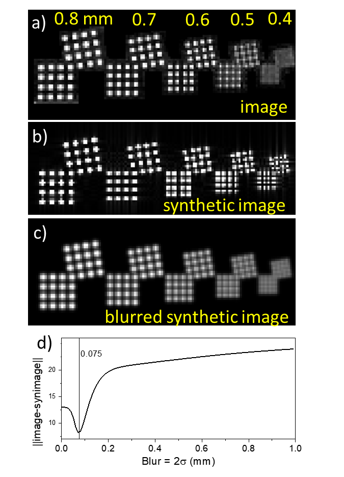
The NIST/ISMRM system phantom (Fig. 1) consists of a 200mm diameter water-filled sphere with a 57-element fiducial array for assessing geometric distortion and image homogeneity; two 14-element arrays for characterizing T1 and T2; a 14-element array for characterizing proton density and SNR; slice profile; and resolution insets. The proton spin relaxation time values for the two relaxation-time arrays, one based on NiCl2 and the other on MnCl2 solutions, are shown in Fig. 1d, along with some reference values for tissue(6). Relaxation time measurements have been discussed previously(7). Here, we focus on geometric distortion, slice profile, resolution, proton density and SNR. Three-dimensional geometric distortion analysis is done by isolating the 57 high-contrast fiducial spheres and determining the sphere center locations using cross correlation and center of mass techniques(8). The scanner-to-phantom coordinate transformation and image uniformity are determined in the same analysis. The slice profile inset consists of a pair of oppositely oriented wedges and conforms to the National Equipment Manufacturers Association (NEMA) standards(9). The resolution inset, based on the ACR phantom(10), consists of hole arrays with hole sizes ranging from 0.8mm to 0.4mm diameter.RESULTS
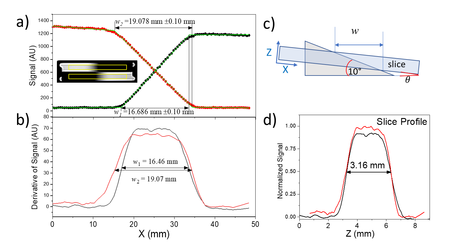
Fig. 2a,b shows the process for determining geometric distortion due to gradient nonlinearity. A 3D gradient echo image is obtained, the fiducial spheres are isolated, and sphere centers are determined. Fig. 2c shows the results of geometric distortion analysis with and without the nonlinear gradient corrections, showing maximal distortion of approximately 2% without corrections and 1% with corrections. Fig. 3 shows results of slice thickness and slice profile measurements using the NEMA protocol and a modified automated analysis. Here, the measured slice thickness was 3.15mm and 3.16mm ±0.2 mm for the two analyses, while the prescribed slice thickness was 3.0mm. Fig. 4 shows automated resolution inset analysis, which consists of generating a synthetic k-space image and applying a k-space point spread function until the difference between the real-space image and synthetic image is minimized. For the scan shown, with a voxel size of 0.35mm, the manual ACR method yields a resolution of 0.5mm, while the automated analysis reports a protocol-based resolution contribution, due to finite k-space sampling, of 0.35 mm, and an additional scanner-based contribution of 0.075 mm. Fig. 5 shows results from a proton density measurement and an SNR analysis. Using a local background reference, the proton density measurement accuracy is less than 10%. Two SNR analyses, one measuring temporal and the other spatial noise, are shown. The first calculates noise from the difference of two identical sequential images, the second from the standard deviation within a uniform region of interest (ROI).DISCUSSION
Geometric distortion analysis is important to provide uncertainty in distance and volume measurements. Typical measured distortions from nonlinear gradients are 2% over a 200mm spherical volume, going below 1% with accurate corrections. Verifying and recording nonlinear gradient corrections is required for use in further corrections to gradient based measurements, such as diffusion and flow. The slice thickness and profile measurements are important to verify that the scanner is operating according to specification, and knowledge of the slice profile is required for implementing corrections to flip angle dependent measurements such as for many T1 and T2 protocols. For the scan shown in Fig. 3, 30% of the signal comes from the slice edges, where the flip angles may be non-ideal.CONCLUSION
Here we have shown how the ISMRM/NIST system phantom can be used for basic scanner diagnostics assessing geometric distortion, image homogeneity, SNR, resolution and slice profile. The resulting data can provide both parameters to benchmark scanner performance and insight on what is determining these parameters. For example, resolution analysis can separate the pulse-sequence component from the intrinsic scanner component of the point spread function. The SNR protocol can separate temporal and spatial noise components, which contribute in different ways to SNR. Finally, the MR-parameter arrays provide a broad range of properties to allow validation of both standard and advanced quantitative protocols.Acknowledgements
We thank Michael Snow and William Hollander at High Precision Devices for the computer aided design and manufacturing guidance. We thank Elizabeth Mirowski from Verellium and Joshua Levy from Phantom Labs for useful discussions on phantom design and implementation. We thank Dr. Paul Finn from UCLA for his continued encouragement and suggestions. We thank all of the ISMRM SQMR committee members, past and present, for their advice and support.
References
1. Russek SE, Boss M, Jackson EF, Jennings DL, Evelhoch JL, Gunter JL, Sorensen AG. Characterization of NIST/ISMRM MRI System Phantom. Proc Intl Soc Mag Reson Med 20, 2012:2456.
2. Boss MA, Dienstfrey AM, Gimbutas Z, Keenan KE, Splett JD, Stupic KF, Russek SE. Magnetic Resonance Imaging Biomarker Calibration Service: Proton Spin Relaxation Times. NIST SP250-97; 2018.
3. Jiang Y, Ma D, Keenan KE, Stupic KF, Gulani V, Griswold MA. Repeatability of magnetic resonance fingerprinting T1 and T2 estimates assessed using the ISMRM/NIST MRI system phantom. Magnetic Resonance in Medicine. 2017;78(4):1452-1457. doi: 10.1002/mrm.26509. PubMed PMID: 27790751; PMCID: PMC5408299.
4. Keenan KE, Gimbutas Z, Dienstfrey A, Stupic KF. Assessing effects of scanner upgrades for clinical studies. Journal of Magnetic Resonance Imaging. 2019;0(0). doi: 10.1002/jmri.26785.
5. Bane O, Hectors SJ, Wagner M, Arlinghaus LL, Aryal MP, Cao Y, Chenevert TL, Fennessy F, Huang W, Hylton NM, Kalpathy-Cramer J, Keenan KE, Malyarenko DI, Mulkern RV, Newitt DC, Russek SE, Stupic KF, Tudorica A, Wilmes LJ, Yankeelov TE, Yen Y-F, Boss MA, Taouli B. Accuracy, repeatability, and interplatform reproducibility of T1 quantification methods used for DCE-MRI: Results from a multicenter phantom study. Magnetic Resonance in Medicine. 2018;79(5):2564-75. doi: 10.1002/mrm.26903.
6. IT’IS. Database of Tissue Properties: Foundation for Research on Information Technologies in Society. Available from: https://itis.swiss/virtual-population/tissue-properties/database/relaxation-times/.
7. Keenan KE, Stupic KF, Boss MA, Russek SE, Chenevert TL, Prasad PV, Reddick WE, Cecil KM, Zheng J, Hu P, Jackson EF. Multi-site, multi-vendor comparison of T1 measurement using NIST/ISMRM system phantom. Proc Intl Soc Mag Reson Med 24, 2016:3290.
8. Gunter JL, Bernstein MA, Borowski BJ, Ward CP, Britson PJ, Felmlee JP, Schuff N, Weiner M, Jack CR. Measurement of MRI scanner performance with the ADNI phantom. Med Phys. 2009;36(6):2193-205. Epub 2009/07/21. doi: 10.1118/1.3116776. PubMed PMID: 19610308; PMCID: PMC2754942.
9. NEMA. Standards Publication MS 5-2018 Slice Thickness. Determination of Slice Thickness in Diagnostic Magnetic Resonance Imaging. 2018.
10. ACR. Phantom Test Guidance for Use of the Large MRI Phantom for the ACR MRI Accreditation Program. American College of Radiology; 2018.
Figures