Introduction

Recently, image processing methods, termed amplified MRI (aMRI), have been introduced to visualize small sub-pixel motions that are too small to see with naked eyes (1, 2), based on methods developed for video processing (3). Potential factors affecting the outcomes include number of image frames for one cycle of movement, the motion amplification bandwidth, the size of movement relative to the pixel size, and the SNR of MR images. Here computer simulations were conducted to investigate how the accuracy of the quantification of motions depended on various parameters. .

Method

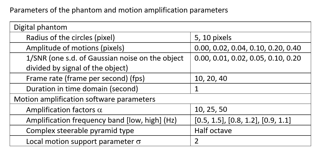
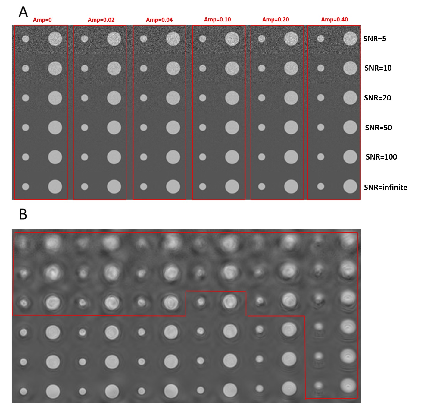
Digital Phantom A series of 2D images contained solid circles in non-zero background with sub-pixel sinusoidal motions. Table 1 lists the parameters of the digital phantom. There was gaussian noise in the objects and background. First, we simulated the k-space MRI data (512x256 matrix size) and then calculated the MRI for each image frame of the digital phantom. The simulations included the Gibbs ringing effects inherent in MRI. Amplitude images containing Gaussian noise were used for testing the motion amplification software. One example of the simulated MR image is shown in Figure 1A.

Motion Amplification The motion amplification used a phase-based motion amplification software in MATLAB (3). Table 1 also contains parameters used in the motion amplification processing.

Image Analysis The image analyses were conducted using internally written software in IDL. A binary mask was generated for each circle at the half of signal level. The position of the center of mass was calculated to present the movement. The positions in the whole motion cycle were fit to a sine function to obtain the amplitude and residual error (deviation from a sine wave).
The measured amplitude was compared with the theoretical value. To evaluate the accuracy of the motion amplification, a relative percentage error (Err%) was calculated as

Err%=\frac{\Amplitue_{ampl}-alpha\cdotAmplitude_{true}}{alpha\cdotAmplitude_{true}}

where α is the amplification factor, Amplitude_true is the actual oscillation amplitude, and Amplitude_ampl is the oscillation amplitude after motion amplification.

Motion amplified image series were inspected visually to exclude objects that lost the sharpness of the boundary from entering statistical analysis.

Statistical Analysis R was used for statistical analysis and plots.

Results

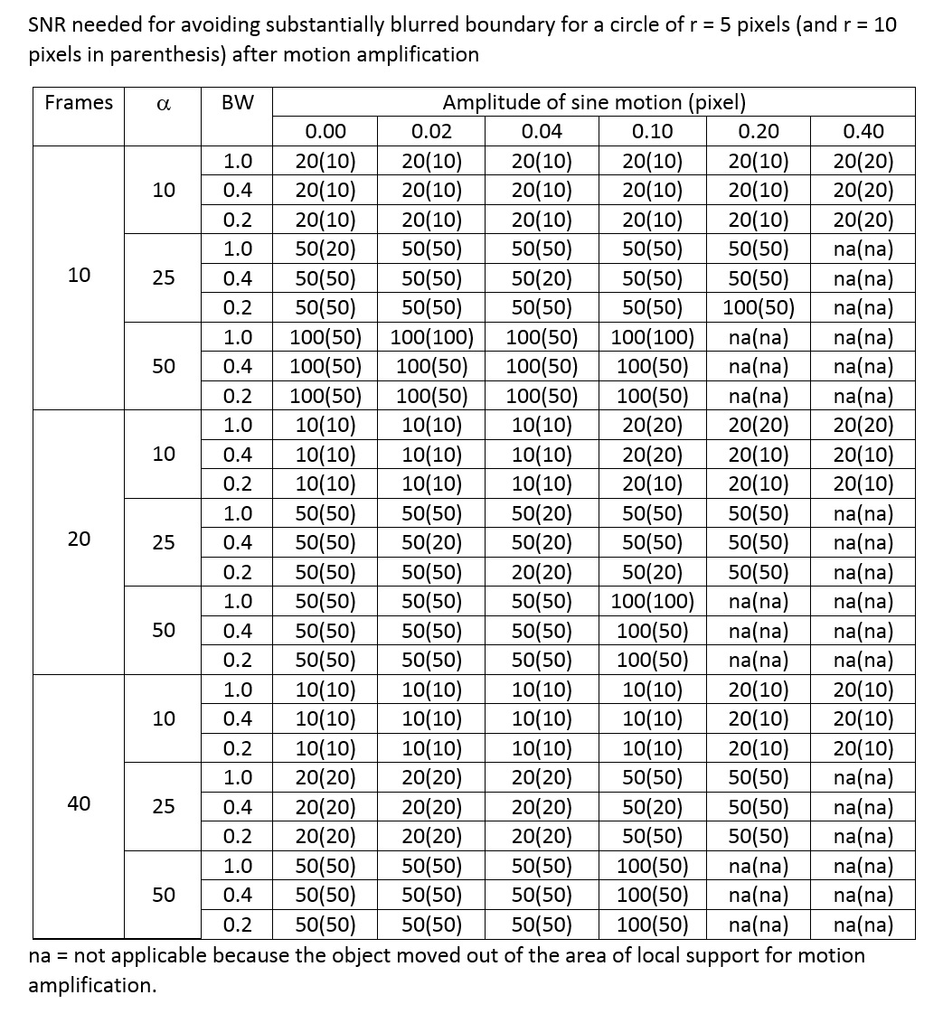
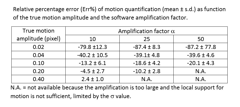
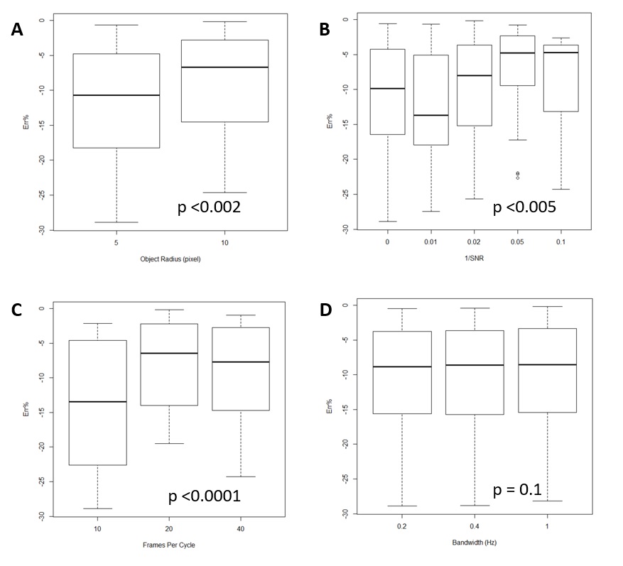
At low SNR, the motion-amplified objects lost the sharpness of the boundary and became substantially burred (Figure 2B). At large amplification factor and for objects with more motion, the motion-amplified object moved out of the local support (3) and the objects also became distorted. Table 2 lists the SNR needed for the circular objects to maintain a reasonably sharp boundary throughout the cycle of sinusoidal movement when the object stayed within the local support. Time course of these “well-behaved” objects followed a sine wave displacement pattern with low residual errors. For motionless objects, the software returned a small amount of motion. The peak displacement was no more than one pixel in the motion-amplified images in the parameter range tested.

The accuracies of quantifying small motions are listed in Table 3. With the motion amplitude of 0.02 and 0.04 pixels, the amplified movement amplitude was expected to be in the range of 0.2 to 2 pixels. The relative error was quite large and motion was under-estimated. When the amplitude of oscillation was 0.1 pixels or more, the errors were in general no more than 20%, and could be as low as a few percent. The sensitivity of the relative error to various factors is explored in Figure 2. The larger object had smaller Err% values. Using 20 or 40 image frames per cycle was better than using 10 frames. Furthermore, as long as the boundary remained sharp, higher SNR did not help to reduce the error. Finally, the bandwidth did not affect the outcome.

Discussion and Conclusions

This work explored the range of various parameters for aMRI to work optimally. The SNR, frame rates and the amplification factor affected whether the boundaries of the object were preserved. However, provided the boundaries of the objects were well preserved after amplification, the quantification accuracy was not sensitive to SNR.

Our computer simulation suggests that this method can be used to quantify small motion with reasonable accuracy for MR images. The aMRI approach opens up many potentially important applications.

References

1. Terem I et al, Revealing sub-voxel motions of brain tissue using phase-based amplified MRI (aMRI), MRM 2018;80(6):2549-2559
2. Hahn S et al, Assessment of cardiac‐driven liver movements with filtered harmonic phase image representation, optical flow quantification, and motion amplification, MRM 2019;81(4):2788-2798
3. Wadhwa N, Rubinstein M, Durand F, Freeman WT. Phase-based video motion processing. ACM Trans Graph. (Proceedings SIGGRAPH 2013), 2013;32.