3345
Machine learning based Magnetic tracking technique using a Mapping of the Magnetic Gradient Fields on a 3T MRI scanner1IADI, U1254, INSERM, Nancy, France, 2Université de Lorraine, Nancy, France, 3FHNW, University of Applied Sciences and Arts Northwestern Switzerland, Muttenz, Switzerland, 4Metrolab Technology SA, Plan-les-Ouates, Switzerland
Synopsis
This paper presents a magnetic tracking method for the localization of a three-axis magnetometer within an MRI bore (Prisma, Siemens, Erlangen, Germany). The unique relationship between the Magnetic Gradient Fields (MGF) and the position within the bore allows locating the sensor through the use of a mapping of the MGF. This mapping is used for the training of a multi-layer perceptron neural network, which estimates the position of the sensor when measuring the MGF. Our technique was experimentally validated by moving the sensors within the MRI bore while playing a customized pulse sequence and by reconstructing the movements during post-processing.
Introduction
Localizing sensors within a magnetic field is a commonly used technique in industrial and biomedical applications. Magnetic tracking can be used for example in the growing field of interventional MRI1 or electrophysiology2. The unique relationship between Magnetic Gradient Fields (MGF) and the localization allows one to locate a magnetic sensor within the MRI bore during an imaging pulse sequence. A magnetic field sensor system compatible with a 3T-MRI environment providing full field vector information was previously presented and validated through the measurements of the static magnetic field and MGF within an MRI bore3.Purpose
This paper presents a magnetic tracking method based on a multilayer perceptron (MLP) neural network. The command signals of each individual gradient coil are available through a homemade solution, the Signal Analyzer and Event Controller (SAEC)4. These command signals and the magnetic sensor measurements are then used to estimate the sensor position using the mapping of the MGF.Methods
The magnetic sensor device consists of a three-axis magnetometer on a chip (Metrolab Technology SA, Switzerland)5.The sensor allows measuring the 3T static magnetic field as well as the MGF. The system’s effective number of bits was set to 16 bits, thus allowing field changes of approximately 92 µT on top of a 3T baseline to be detected.
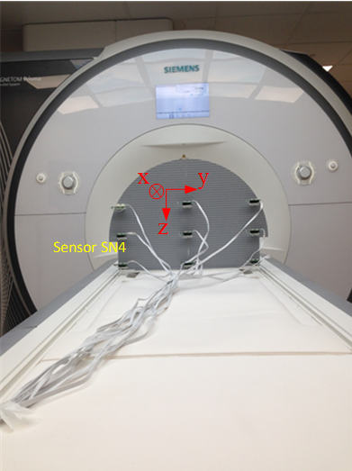
The acquisitions for the mapping of the MGF were performed on a 3T MRI scanner (Prisma, Siemens, Erlangen, Germany) (Fig. 1). 9 sensors were mounted on a Lego® plate6 and aligned with the MRI axis. Several sets of measurements were performed as the MRI table was moved outwards from z=0mm to z=300mm every 25mm (117 points).
Those measurements were used to train an MLP taking as input the three normalized gradient measurements and outputting the position coordinates within the MRI bore. By combining the command signals from the SAEC during an MRI sequence and the magnetic profile map of individual gradient coils, one can use the unique relationship (function estimated by the MLP) between the localization of the sensor and the gradient information.
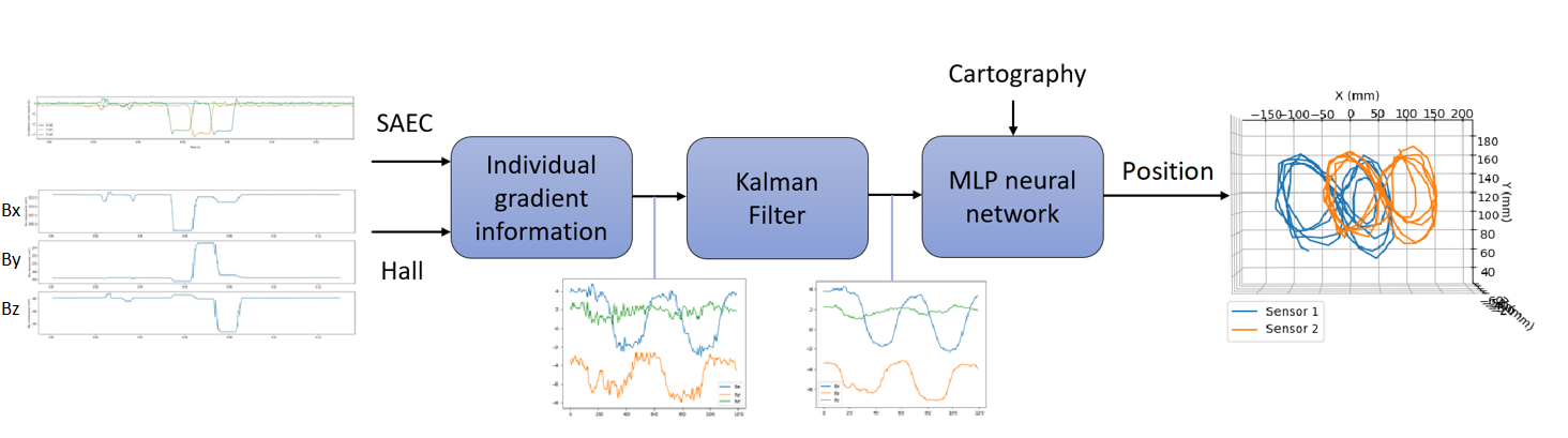
A custom pulse sequence consisting of successive individual gradient plateaus was played as the sensor was moved inside the MRI bore. The MGF measurements were extracted and normalized thanks to the command signals acquired by the SAEC. The gradient information was smoothed through a Kalman Filter before being fed into the MLP. The flowchart of the algorithm is depicted in figure 2.
Given the lack of a reference, our algorithm was assessed by moving two sensors separated by a constant distance d. A whole set of periodic movements were made at different locations within the MRI tunnel. The movements covered displacements along the three different axes with different speeds and amplitudes, and following simple geometric shapes. The movements were estimated using the algorithm described above, the distance d’ between the two estimated positions was computed at each timestep and compared with the real distance d separating the sensors.
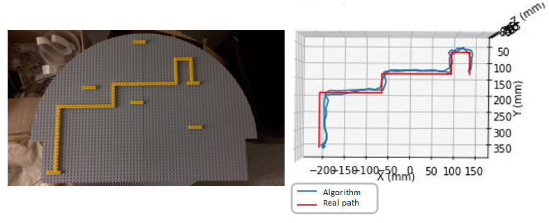
Another set of experiments consisted of a single sensor being moved along a path marked with Lego® bricks on the Lego® plate, as shown in figure 4.
Results
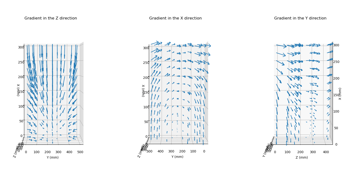
Figure 3 shows the mapping of the MGF obtained with our system. A MLP network was trained to link the mapping of MGF (Gx,Gy,Gz) to the position of the sensor (x,y,z).A mean absolute error of 0.499 ± 0.392 cm between the estimated distance d’ and the real distance d was reported. (95% confidence interval (CI): [0.021, 1.457] cm)
Figure 4 shows the path along which the sensor was moved at almost constant speed (in red) and the movement reconstruction (in blue). The initial position of the sensor is known and the speed along the path is considered constant by parts for integration purposes, leading to an absolute error of 1.371 ± 0.456 cm, ( 95% CI : [ 0.530, 2.200] cm )
Discussion
The results are promising and seem to indicate a localization precision under 2 cm. However, these results were obtained without a gold-truth reference, as no validated tracker was used to assess the proposed technique. Further tests are therefore required using a previously validated position tracker such as a camera-based technique.The current tests were performed using a custom pulse sequence consisting of consecutive plateaus of gradients in each direction. This sequence allowed us to provide all the information required for the tracking. Further improvements are required in order to ensure that tracking will be possible while playing clinically used pulse sequences, without needing the need of additional gradients being played.
Conclusion
The mapping of the MGF allowed the creation of a database, which was later used to train a neural network able to localize a magnetic sensor within the MRI bore with a resolution of 2 centimeters (while a custom pulse sequence is being played). To our knowledge, it is unique in its approach of using machine learning to perform magnetic tracking based on a mapping of the gradient fields.Acknowledgements
We gratefully acknowledge the support of NVIDIA Corporation with the donation of the Titan XP GPU used for this research.References
[1] SCHELL, J.-B., KAMMERER, J.-B., HÉBRARD, Luc, et al. Towards a Hall effect magnetic tracking device for MRI. In : 2013 35th Annual International Conference of the IEEE Engineering in Medicine and Biology Society (EMBC). IEEE, 2013. p. 2964-2967.
[2] Amiran S. Revishvili, Erik Wissner, Dmitry S. Lebedev, Christine Lemes, Sebastian Deiss, Andreaas Metzner, Vitaly V. Kalinin, Oleg V. Sopov, Eugeny Z. Labartkava, Alexander V. Kalinin, Michail Chmelevsky, Stephan V. Zubarev, Maria K. Chaykovskaya, Mikhail G. Tsiklauri, Karl-Heinz Kuck, "Validation of the mapping accuracy of a novel non-invasive epicardial and endocardial electrophysiology system", EP Europace, Volume 17, Issue 8, August 2015, Pages 1282–1288
[3] Joris Pascal, Nicolas Weber, Jacques Felblinger, Julien Oster " Magnetic gradient mapping of a 3T MRI scanner using a modular array of novel three-axis Hall sensors “, ISMRM 2018, Paris, Abstract #1759
[4] Odille F, Pasquier C, Abacherli R, Vuissoz PA, Zientara GP, Felblinger J. Noise cancellation signal processing method and computer system for improved real-time electrocardiogram artifact correction during MRI data acquisition. IEEE Transactions on Biomedical Engineering. 2007 Mar 19;54(4):630-40.
[5] Metrolab Technology SA, MagVector™ MV2 3-axis magnetic sensor, Datasheet, v 2.1 r 1.0 – 07/2016
[6] SCHELL, J., KAMMERER, J., HÉBRARD, L., et al. 3T MRI scanner magnetic gradient mapping using a 3D Hall probe. In: Sensors, 2012 IEEE. IEEE, 2012. p. 1-4.
Figures