3299
A Learning-From-Noise Dilated Wide Activation Network for Denoising Arterial Spin Labeling (ASL) Perfusion Images1Temple University, Philadelphia, PA, United States, 2University of Maryland School of Medicine, Philadelphia, MD, United States
Synopsis
In this study, we showed that without a noise-free reference, Deep Learning based ASL denoising network can produce cerebral blood flow images with higher signal-to-noise-ratio (SNR) than the reference. In this learning-from-noise training scheme, cerebral blood flow images with very high noise level can be used as reference during network training. This will remove any deliberate pre-processing step for getting the quasi-noise-free reference when training deep learning neural networks. Experimental results this learning-from-noise training scheme preserved the genuine cerebral blood flow information of individual subjects while suppressed noise.
Introduction
Arterial spin labeling (ASL) perfusion MRI provides a non-invasive way to quantify cerebral blood flow (CBF) but it still suffers from an inherently low signal-to-noise-ratio (SNR). Recently, deep machine learning (DL) has been adopted for ASL CBF denoising and shown promising results[2,7,9]. Even without a noise-free reference, DL-based ASL denoising network (ASLDN) proposed thus far [7,8] can produce CBF images with higher SNR than the reference, suggesting a learning-from-noise capability of DL [1]. In fact, if the ASLDN is configured to minimize the mean square error (MSE) between the reference and the projected input (the loss function), it is to find the optimum at the arithmetic mean of the observations if both the input and the reference are drawn from the same distribution [1]. This process matches well with the need of pursuing an optimal average out of all acquired CBF map time series. The purpose of this study was to testify whether an ASLDN can be built from network specifically designed for learning-from-noise so CBF images with the same or similar noise level can be used as reference during network training, which will remove any deliberate pre-processing step for getting the quasi-noise-free reference. We dubbed this new method as ASLDN-LFN.Methods
ASL data were pooled from 280 subjects in a local database. The data were acquired with a pseudo-continuous ASL sequence (40 label/control (L/C) image pairs with labeling time = 1.5 sec, post-labeling delay = 1.5 sec, FOV=22x22 cm2, matrix=64x64, TR/TE=4000/11 ms, 20 slices with a thickness of 5 mm plus 1 mm gap). Image processing was performed with ASLtbx [6] using the latest processing steps [5]. The resulting mean CBF images (of 10 or the 40 pairs) were spatially normalized into the Montreal Neurological Institute (MNI) space. Every 3 slices from the 35th to the 59th axial slices were extracted from each of the 3D CBF image. The Dilated Wide Activation Network (DWAN) [8] (shown in Figure 1) was used to build ASLDN-LFN. CBF image slices from 200 subjects were used as the training dataset. CBF images from 20 different subjects were used for validation. The remaining 60 subjects were used as the testing set. Input to ASLDN-LFN was the axial slice. The 40 ASL CBF images of each subject were divided into 4 time segments, each with 10 successively acquired images. The mean maps of the 1st segment and the 2nd segment were taken as the input and the corresponding reference for DL model training. Another set of input-reference image pairs were obtained from the mean CBF maps of the 3rd and the 4th segment. During model testing, the mean CBF image slices of the first 10 L/C pairs (in the first time segment) were used as the input.Method performance was measured by SNR and Grey Matter/White Matter (GM/WM) contrast ratio of the output CBF maps. SNR was calculated by using the mean signal of a grey matter (GM) region-of-interest (ROI) divided by the standard deviation of a white matter (WM) ROI in slice 50. GM/WM contrast was calculated as the mean value of GM masked area divided by the mean value of WM masked area. Correlation coefficient at each voxel between the DL-processed CBF values and the CBF value derived from the entire 40 L/C pairs processed by the non-DL methods listed in [5].
Results
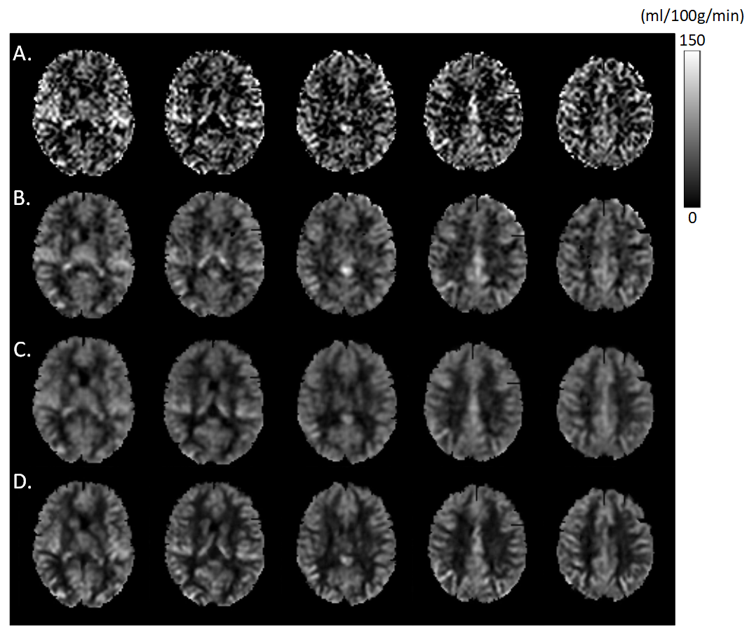
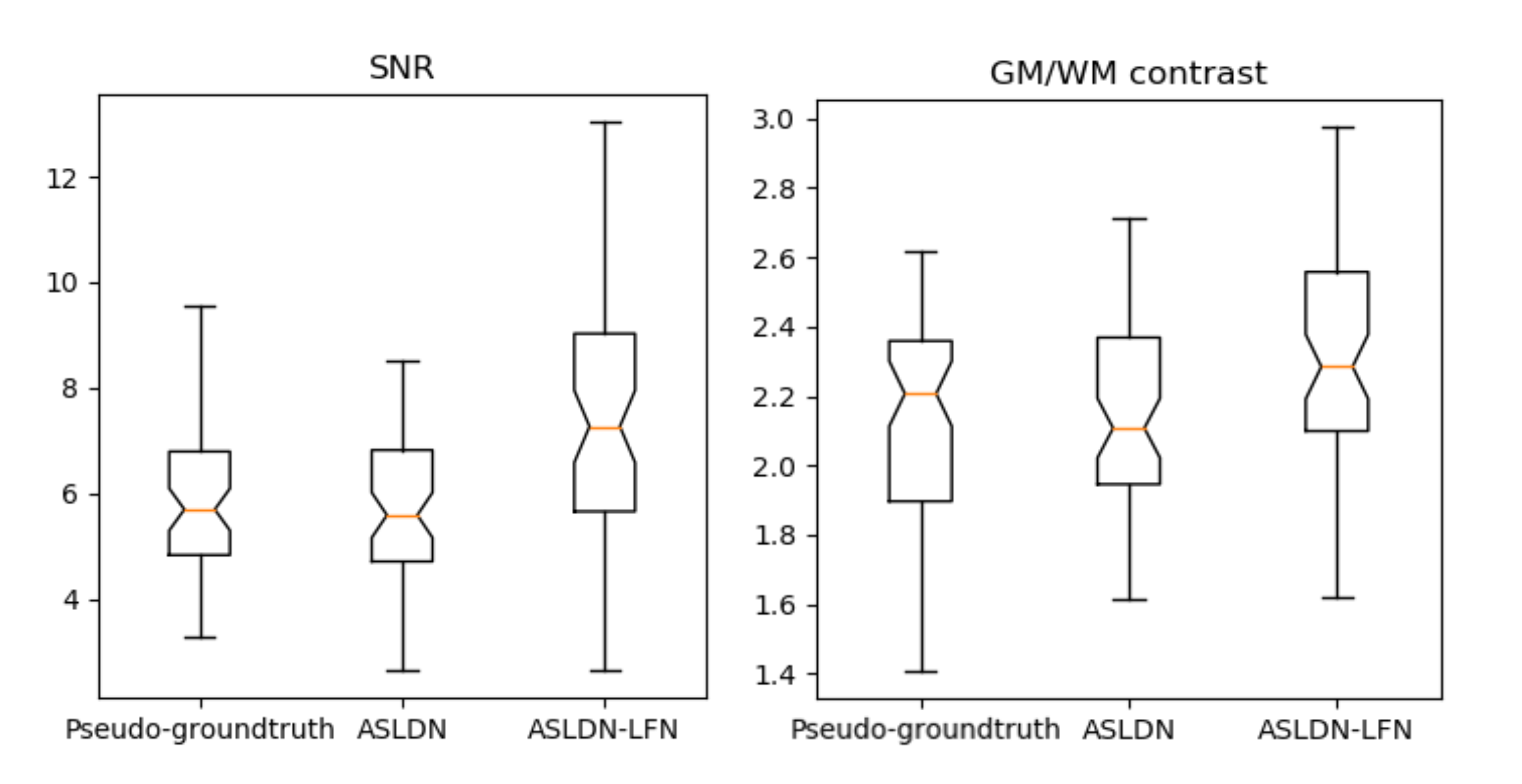
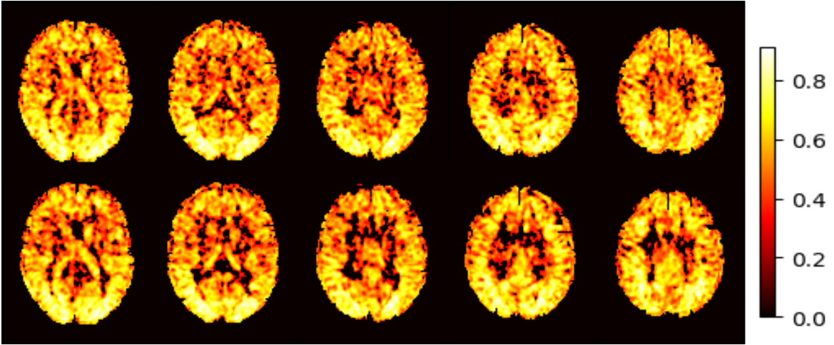
Figure 2 shows the mean CBF maps produced by different algorithms. ASLDN-LFN (Fig. 2.D) showed the best CBF image quality. Figure 3 shows the notched box plot of the SNR and GM/WM contrast ratio based on the testing data from the 60 subjects. Average SNR was 5.87, 6.36, and 8.06 for the pseudo-groundtruth (mean CBF map derived from the 40 L/C pairs), ASLDN, and ASLDN-LFN, respectively. The average GM/WM contrast was 2.14, 2.15, and 2.32 for the pseudo-groundtruth, the output of ASLDN and the output of ASLDN-LFN, respectively. ASLDN-LFN improved SNR by 26.7% and improved GM/WM contrast by 7.9% compared to our previous ASLDN. Figure 4 shows that both the CBF values output by ASLDN and ASLDN-LFN were highly correlated to those of the pseudo-groundtruth.Discussion and conclusion
ASLDN-LFN was proposed to denoise ASL CBF images under the supervision of low SNR reference. Our results demonstrated that ASLDN-LFN achieved similar or even better denoising effects than our previous ASLDN in terms of SNR and GM/WM contrast. CBF value produced by ASLDN-LFN was highly correlated to that of the pseudo-groundtruth, meaning that ASLDN-LFN preserved the genuine CBF information of individual subjects while suppressed noise. The better performance of ASLDN-LFN may be attributed to the “learning-from-noise” property of the deep network as well as the increased training sample size because fewer L/C pairs were required to generate the reference image, allowing more training data to be extracted from the same ASL image series.Acknowledgements
This work was supported by NIH/NIA grant: 1 R01 AG060054-01A1References
[1] Lehtinen, Jaakko, et al. "Noise2Noise: Learning Image Restoration without Clean Data." International Conference on Machine Learning. 2018. [2] Kim, Ki Hwan, Seung Hong Choi, and Sung-Hong Park. "Improving Arterial Spin Labeling by using deep learning." Radiology 287.2 (2017): 658-666. [3] Yu, Jiahui, et al. "Wide activation for efficient and accurate image super-resolution." arXiv preprint arXiv:1808.08718 (2018). [4] Shin, David D., et al. "Pseudocontinuous arterial spin labeling with optimized tagging efficiency." Magnetic resonance in medicine 68.4 (2012): 1135-1144. [5] Li, Yiran, et al. "Priors-guided slice-wise adaptive outlier cleaning for arterial spin labeling perfusion MRI." Journal of neuroscience methods 307 (2018): 248-253. [6] Wang, Ze, et al. "Empirical optimization of ASL data analysis using an ASL data processing toolbox: ASLtbx." Magnetic resonance imaging 26.2 (2008): 261-269. [7] Xie, Danfeng, Li Bai, and Ze Wang. "Denoising Arterial Spin Labeling Cerebral Blood Flow Images Using Deep Learning." arXiv preprint arXiv:1801.09672 (2018). [8] Xie, Danfeng, et al. "BOLD fMRI-Based Brain Perfusion Prediction Using Deep Dilated Wide Activation Networks." International Workshop on Machine Learning in Medical Imaging. Springer, Cham, 2019. [9] Gong, Enhao et al. "Boosting SNR and/or resolution of arterial spin label (ASL) imaging using multi-contrast approaches with multi-lateral guided filter and deep networks," in 25th Annual Meeting of the International Society for Magnetic Resonance in Medicine, Honolulu, 2017. [10] F. Yu and V. Koltun, "Multi-scale context aggregation by dilated convolutions," arXiv preprint arXiv:1511.07122, 2015.Figures
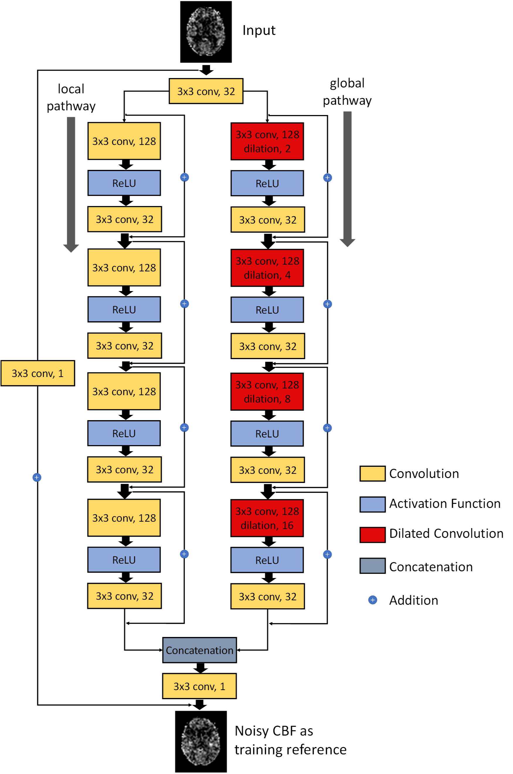
Figure 1: Illustration of the architecture of DWAN. The output of the first layer was fed to both local pathway and global pathway. Each pathway contains 4 consecutive wide activation residual blocks. Each wide activation residual block contains two convolutional layers (3×3x128 and 3×3x32) and one activation function layer. The 3x3x128 convolutional layers in the global pathway were dilated convolutional layers [10] with a dilation rate of 2, 4, 8, 16, respectively (a×b×c indicates the property of convolution. a×b is the kernel size of one filter and c is the number of the filters).