Introduction

Perfusion imaging evaluates the blood flow through the tissue capillary bed¹,which is an important biomarker of tissue vitality. Current quantification of perfusion is based on Kety’s equation,which requires a global arterial input function (AIF), making perfusion quantification highly dependent on the selection of the arterial region, its size, shape, and location. Quantitative transport mapping (QTM) eliminates the AIF problem by computing a velocity and flow field based on the transport equation of mass flux^2,3. QTM is applied to time resolved contrast enhanced data to map cerebral blood flow (CBF). Here we use multi-delay ASL data and compare CBF obtained using QTM and the traditional Kety method.

Methods

Algorithm:
Given multi-delay ASL data $$$c(\xi,t_i)$$$ for voxels $$$\xi$$$ at times $$$t_i$$$, QTM solves the following transport inverse problem:$$\boldsymbol{q}=argmin_{\boldsymbol{q}}\sum_{i=1}^{N}||c_{t}(\xi,t_{i})+\nabla\cdot \frac{c_{t}(\xi,t_{i})\boldsymbol{q}(\xi)}{V\cdot CBV(\xi)} ||_{2}^{2}+\lambda||\boldsymbol{q}||_{2}^{2} \qquad (1)$$ with $$$c_{t}(\xi,t_{i})=\frac{1}{\Delta t}[c(\xi,t_{i+1})-c(\xi,t_{i})]$$$ the temporal derivative of c. $$$\boldsymbol{q}(\xi)=[q^{x}(\xi),q^{y}(\xi),q^{z}(\xi)]$$$ is the flow defined on the three surfaces of the voxel at positive x,y,z directions, $$$CBV(\xi)$$$ is the cerebral blood volume fraction within the voxel, V the voxel volume, and $$$\nabla\cdot \boldsymbol{f}(\boldsymbol{\xi})=\sum_{i=x,y,z}f^{i}(\xi_{i})-f^{i}(\xi_{i-1})$$$ the divergence operator. An L2 regularization is used for denoising. Eq.1 is solved using a conjugate gradient method. $$$\boldsymbol{q}$$$ is assumed to be a steady flow with $$$\nabla\cdot \boldsymbol{q}=0$$$, which renders the optimization of the discretized form of Eq.1 more robust. Eq.1 contains 3 unknowns for each voxel, so at least 4 time points (3 temporal derivatives) are needed to solve Eq.1.
Numerical validation:
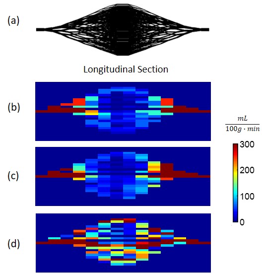
For validating QTM, a vessel tree network in a double-cone shape containing 2560 vessel segments with a 1cm mid cross-section radius and 6 cm length (Fig.1a) was generated using the branching rule⁷. The inlet velocity was set to 2cm/s and plug flow was assumed for each vessel segment in order to simplify the forward problem of generating 4D tracer imaging data of sufficient spatiotemporal resolution using the mass flux equation⁸ (Fig.1b, c and d). The concentration data was simulated using finite element modeling (FEM) of the transport equation with a boundary condition of a concentration profile at the inlet being $$$c(t)=te^{-\frac{t}{5}}$$$. The FEM data was then down-sampled to the ASL voxel size and temporal frame duration and QTM was applied. $$$\lambda=1$$$ was chosen empirically to minimize simulation error and used for both simulation and ASL data.
In vivo imaging experiment.
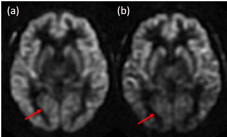
A background suppression pulse was interleaved into the labeling pulse to realize short pulse label delay 3D acquisition⁴. Two methods were used to acquire multi-delay ASL: the first was to fix labeling time (1500ms) and vary post label delay (PLD) (25ms-2525ms with 500ms interval), and the second was to fix PLD (25ms) and vary labeling time (1500ms-4000ms with 500ms interval). The corresponding ASL data is shown in Fig.2. The first method was chosen for better signal in the posterior brain. As the PLDs were smaller than mean transit time (MTT), tracer stayed mainly in artery and capillary space⁵. Therefore, CBV was set to the blood volume of artery (CBVa), which was 1% for gray matter and 0.75% for white matter⁶. A T1w image was used to generate gray/white matter segmentation and the CBV value for each voxel. 7 healthy subjects were scanned on a 3T GE scanner, using the PCASL sequence (voxel size mm³, field of view 24cm, number of slices 36, 6 post label delays). The flow vector $$$\boldsymbol{q(\boldsymbol{\xi})}(mm^{3}/s)$$$ from QTM was converted to CBF (in mL/100g/min) using: $$CBF=\frac{\sqrt{q^x(\xi)^2+q^y(\xi)^2+q^z(\xi)^2}}{\rho V}\cdot 100g\cdot 60s,$$ where $$$\rho$$$ is blood density. CBF generated using Kety’s method⁹ was used as comparison in both simulation and in vivo data.

Results

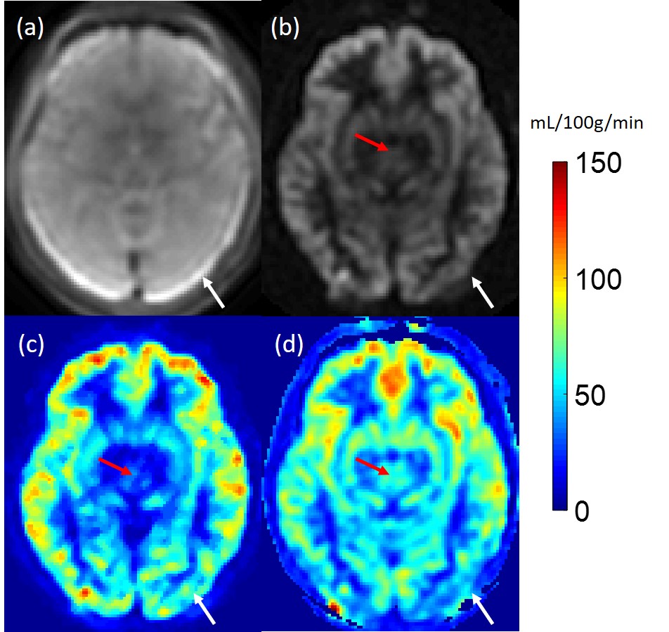
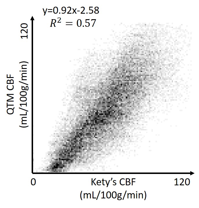
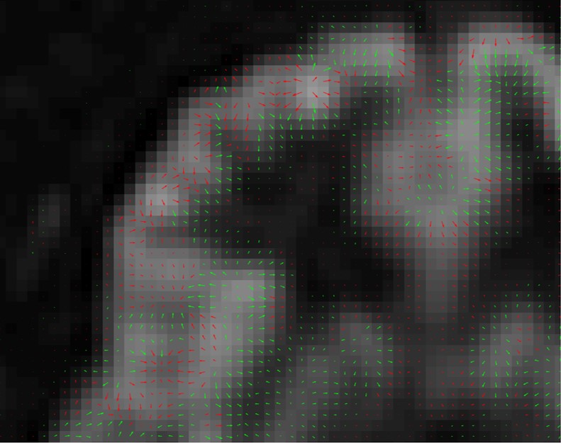
Figure 1 shows high accuracy of QTM flow mapping (Figure 1c), but substantial error in Kety’s flow (Figure 1d). Figure 3 shows an in vivo comparison of CBF obtained using QTM (Figure 3c) and Kety’s method (Figure 3d). Flow using QTM was more uniform in the posterior gray matter, but lower near the circle of Willis, compared to Kety’s flow (Figure 3, arrows). A weak correlation between QTM and Kety’s flow was observed (Figure 4). The average flow in gray matter was 63±15 mL/100g/min for QTM and 65±14 mL/100g/min for Kety’s method, while in white matter it was 42±17 mL/100g/min for QTM and 46±14 mL/100g/min for Kety’s method. Figure 5 shows the QTM flow vector map overlayed onto the tracer concentration map. QTM captured the in-plane flow from gray matter into white matter, while the flow vertical to the plane needs to be validated because the slice thickness is large (4mm).

Discussion and Conclusion

In simulation, QTM based flow was more accurate than Kety’s. In healthy subjects, QTM showed a more uniform flow in the posterior gray matter, likely due the Kety method's reliance on the M0 map (Figure 3a) and there is artifact in M0 near the edge of the brain. QTM estimated flow is low near the circle of Willis, possibly due the inability to capture flow in large arteries with the used frame rate. While QTM and Kety’s method produced similar average flow for global gray and white matter, QTM flow vector map captures blood flow from gray matter to white matter. Further validation using flow phantoms and more realistic vasculature models are warranted to evaluate the QTM flow vector map.

References

1. Kety SS. The theory and applications of the exchange of inert gas at the lungs and tissues. Pharmacol Rev 1951;3(1):1-41.
2. Zhou L, Spincemaille P, Zhang Q, Nguyen T, Doyeux V, Lorthois S, Wang Y. Vector Field Perfusion Imaging: A Validation Study by Using Multiphysics Model. ISMRM, 2018; Paris, France. p 1870
3. Zhou L, Zhang Q, Spincemaille P, Nguyen T, Wang Y. Quantitative Transport Mapping (QTM) of the Kidney using a Microvascular Network Approximation. ISMRM, 2019 4/26/2019; Montreal. p 703.
4. Dai W, Robson P M, Shankaranarayanan A, et al. Reduced resolution transit delay prescan for quantitative continuous arterial spin labeling perfusion imaging[J]. Magnetic resonance in medicine, 2012, 67(5): 1252-1265.
5. Buxton RB. Introduction to Functional Magnetic Resonance Imaging. Cambridge University Press. (2009) ISBN:1139481304.
6. Hua J, Liu P, Kim T, et al. MRI techniques to measure arterial and venous cerebral blood volume[J]. Neuroimage, 2019, 187: 17-31.
7. Karch R, Neumann F, Neumann M, et al. A three-dimensional model for arterial tree representation, generated by constrained constructive optimization[J]. Computers in biology and medicine, 1999, 29(1): 19-38.
8. Lorthois S, Cassot F, Lauwers F. Simulation study of brain blood flow regulation by intra-cortical arterioles in an anatomically accurate large human vascular network: Part I: methodology and baseline flow. Neuroimage 2011;54(2):1031-1042.
9. Buxton R B. Quantifying CBF with arterial spin labeling[J]. Journal of Magnetic Resonance Imaging: An Official Journal of the International Society for Magnetic Resonance in Medicine, 2005, 22(6): 723-726.