3291
Numerical Approximation to the General Kinetic Model for ASL Quantification1Biomedical Engineering, University of Southern California, Los Angeles, CA, United States, 2Electrical and Computer Engineering, University of Southern California, Los Angeles, CA, United States
Synopsis
We propose a numerical approximation to Buxton's general kinetic model (GKM) for ASL quantification that will enable greater flexibility in ASL acquisition methods. The proposed method combines the Bloch-McConnell equations with the flow effects and hence model the effects of flow simultaneously with magnetization transfer, T2 effects, off-resonance, and irregular timing of labeling. These can be solved using Jaynes’ matrix formalism. The proposed approximation is compared with GKM using simulations for PASL, PCASL, steady-pulse ASL, and MR fingerprinting ASL. Accuracy of the approximation is studied as a function of a key “time interval” parameter using Monte-Carlo simulations.
Introduction
Buxton's general kinetic model (GKM)1 is a widely used ASL quantification method because it is simple, analytic, and provides excellent intuition into signal formation. However, it is nontrivial for GKM to model the effects of flow with magnetization transfer (MT)2,3, T2 effects, off-resonance, and irregular timing of labeling. The aforementioned effects other than flow are efficiently modeled by Jayne's matrix formalism4. In this work, we bridge two methods by adding single compartment inflow and outflow5,6 to the Bloch equations with MT effects7,8,9. We denote these "Bloch-McConnell-Flow" (BMF) equations. We provide numerical approximations to these based on modified Jaynes' matrix formalism.Theory
We assume single-compartment kinetics for perfusion and instantaneous mixing between arterial blood water and tissue. For tissue magnetization (f) and semisolid (s) protons $$$\mathbf{M}(t)=\begin{bmatrix}M_x^f(t) & M_y^f(t) & M_z^f(t) & M_z^s(t) \end{bmatrix}^T$$$ under perfusion, the BMF equations include incoming arterial flow and outgoing venous flow to the tissue compartment of a two-compartment model10 and can be written as $$\frac{d\mathbf{M}(t)}{dt} = \left(\Omega(t)+\Lambda+\Gamma+\Xi\right)\mathbf{M}(t) + \mathbf{D}(t)$$ where $$\Omega(t)=\begin{bmatrix}0 & \gamma \left(\mathbf{G}(t)\cdot\mathbf{r}+\Delta B_0 \right) & -\gamma B_{1,y}(t) & 0\\-\gamma \left(\mathbf{G}(t)\cdot\mathbf{r}+\Delta B_0 \right) & 0 & \gamma B_{1,x}(t) & 0\\ \gamma B_{1,y}(t) & -\gamma B_{1,x}(t) & 0 & 0\\0 & 0 & 0 & -W(\Delta,t)\\\end{bmatrix},\Lambda=\begin{bmatrix} 0 & 0 & 0 & 0\\0 & 0 & 0 & 0\\0 & 0 & -k^f & k^s\\0 & 0 & k^f & -k^s\end{bmatrix},$$$$\Gamma=\begin{bmatrix} -\frac{F}{\lambda} & 0 & 0 & 0\\0 & -\frac{F}{\lambda} & 0 & 0\\0 & 0 & -\frac{F}{\lambda} & 0\\0 & 0 & 0 & 0\end{bmatrix},\Xi=\begin{bmatrix} -\frac{1}{T_2^f} & 0 & 0 & 0\\0 & -\frac{1}{T_2^f} & 0 & 0\\0 & 0 & -\frac{1}{T_1^f} & 0\\0 & 0 & 0 & -\frac{1}{T_1^s}\end{bmatrix},\mathbf{D}(t)=\begin{bmatrix} 0 \\0 \\\left(\frac{1}{T_1^f} + \frac{F}{\lambda}\right)M_0^f + s(t)\\\frac{1}{T_1^s}M_0^s\end{bmatrix},$$$$s(t) = \sum_{i=1}^{M}-\frac{F}{\lambda}M_0 \alpha_0e^{-(t-t_{\ell,i})/T_{1b}}\left(u(t - t_{\ell,i} - T_{D,i}) - u(t - t_{\ell,i} - T_{D,i} - T_{W,i})\right).$$ $$$F$$$ is the blood flow, $$$\lambda$$$ is the tissue-blood partition coefficient, $$$\alpha_0$$$ is the labeling efficiency, $$$T_D$$$ is the transit delay, and $$$T_W$$$ is the bolus duration. Assuming piecewise constant for an RF pulse and $$$s(t)$$$ over a time interval $$$\tau_i$$$ ($$$t_i$$$ is the start time of the $$$i$$$th interval), the system evolves due to rotation as $$$\mathbf{M}(t_i+\tau_i)=\mathbf{R}\mathbf{M}(t_i) $$$ where $$$\mathbf{R}=\mathrm{exp}(\Omega(t_i)\tau_i)$$$ and due to relaxation, clearance, and exchange as11$$\mathbf{M}(t_i+\tau_i)=e^{\left(\Lambda+\Gamma+\Xi\right)\tau_i}\mathbf{M}(t_i)+\int_{t_i}^{t_i + \tau_i} e^{\left(\Lambda+\Gamma+\Xi\right)(t_i+\tau_i-\tau)}\mathbf{D}(\tau)d\tau\cong e^{\left(\Lambda+\Gamma+\Xi\right)\tau_i}\mathbf{M}(t_i)+\left(e^{\left(\Lambda+\Gamma+\Xi\right)\tau_i}-\mathbf{I}\right)\left(\Lambda+\Gamma+\Xi\right)^{-1}\mathbf{D}(t_i).$$ Using a further approximation $$$\Lambda\Gamma\Xi\cong\Gamma\Xi\Lambda$$$, we get $$$\mathrm{exp}((\Lambda+\Gamma+\Xi)\tau_i)\cong\mathrm{exp}(\Lambda\tau_i)\cdot\mathrm{exp}(\Gamma\tau_i)\cdot\mathrm{exp}(\Xi\tau_i)=A(\tau_i)C(\tau_i)E(\tau_i)$$$ where an analytic expression for $$$A(\tau_i)$$$ is given by Gloor et al12. Therefore, we finally obtain the extended Jaynes' matrix formalism$$\mathbf{M}(t_i+\tau_i)=A(\tau_i)C(\tau_i)E(\tau_i)\mathbf{M}(t_i)+(\mathbf{I}-A(\tau_i)C(\tau_i)E(\tau_i))\begin{bmatrix}0\\0\\\left(\frac{1+T_1^sk^s}{1+T_{1app}k^f+T_1^sk^s}\right)(M_0^f+s(t_i)T_{1app})+ \left(\frac{T_{1app}k^s}{1+T_{1app}k^f+T_1^sk^s}\right)M_0^s\\\left(\frac{T_1^sk^f}{1+T_{1app}k^f+T_1^sk^s}\right)(M_0^f+s(t_i)T_{1app})+\left(\frac{1+T_{1app}k^f}{1+T_{1app}k^f+T_1^sk^s}\right)M_0^s\\\end{bmatrix}.$$ Figure 1 shows the extended matrix formalism over the $$$i^{th}$$$ time interval and demonstrates a piecewise constant approximation of labeled blood leads to an overestimation of ASL signal. For the BMF equations without MT effects, we do not need the second approximation since $$$\Gamma\Xi=\Xi\Gamma$$$.The corresponding Jaynes' matrix formalism can be obtained by setting $$$M_0^s=0,k^f=0,k^s=0,A(\tau_i)=\mathbf{I}$$$.
Methods
In this work, we validate the BMF equations without MT effects. The proposed numeric approximation was first compared with GKM for single-compartment kinetics with pulsed labeling and pseudo-continuous labeling. For both labeling methods, recommended labeling parameters were obtained from the recent consensus paper by Alsop et al13. For GKM, PASL and PCASL signals were calculated by evaluating Equations 3 and 5 of Buxton et al1, respectively. We also investigated the effect of the time interval ($$$\tau$$$) on the accuracy of the approximation. We tested 500 time intervals linearly spaced from 0 to 50 msec in increments of 0.1 msec. ASL signals with inversion labeling were generated with GKM ($$$\Delta \mathrm{M}_{GKM}(t))$$$ and the numeric approximation ($$$\Delta \mathrm{M}_{numeric}(t))$$$ while sweeping parameters for transit delay and bolus duration: $$$T_D$$$=(500:1:1500)ms, $$$T_W$$$=(500:10:1000)/(1500:10:2000)ms for PASL/PCASL. Other fixed parameters were $$$F$$$=0.8 (mL/g/min), $$$T_1/T_{1b}/T_2$$$=1820/1650/$$$\infty$$$ms, $$$\Delta f$$$=0, $$$\lambda$$$=0.9. The accuracy of the numeric approximation was assessed using two metrics: (1) overall normalized root-mean-square error (NRMSE)=$$$||\Delta \mathrm{M}_{GKM}(t)-\Delta \mathrm{M}_{numeric}(t)||_2/||\Delta \mathrm{M}_{GKM}(t)||_2$$$, and (2) maximum deviation between GKM and the numeric approximation (Max Deviation)=$$$\mathrm{max}|\Delta \mathrm{M}_{GKM}(t)-\Delta \mathrm{M}_{numeric}(t)|$$$. To demonstrate the generality of the proposed method, we validated the numeric approximation against steady-pulsed ASL (spASL)14,15,16 and MR fingerprinting ASL (MRF-ASL)17, where theoretical signal expressions are derived with GKM.Results
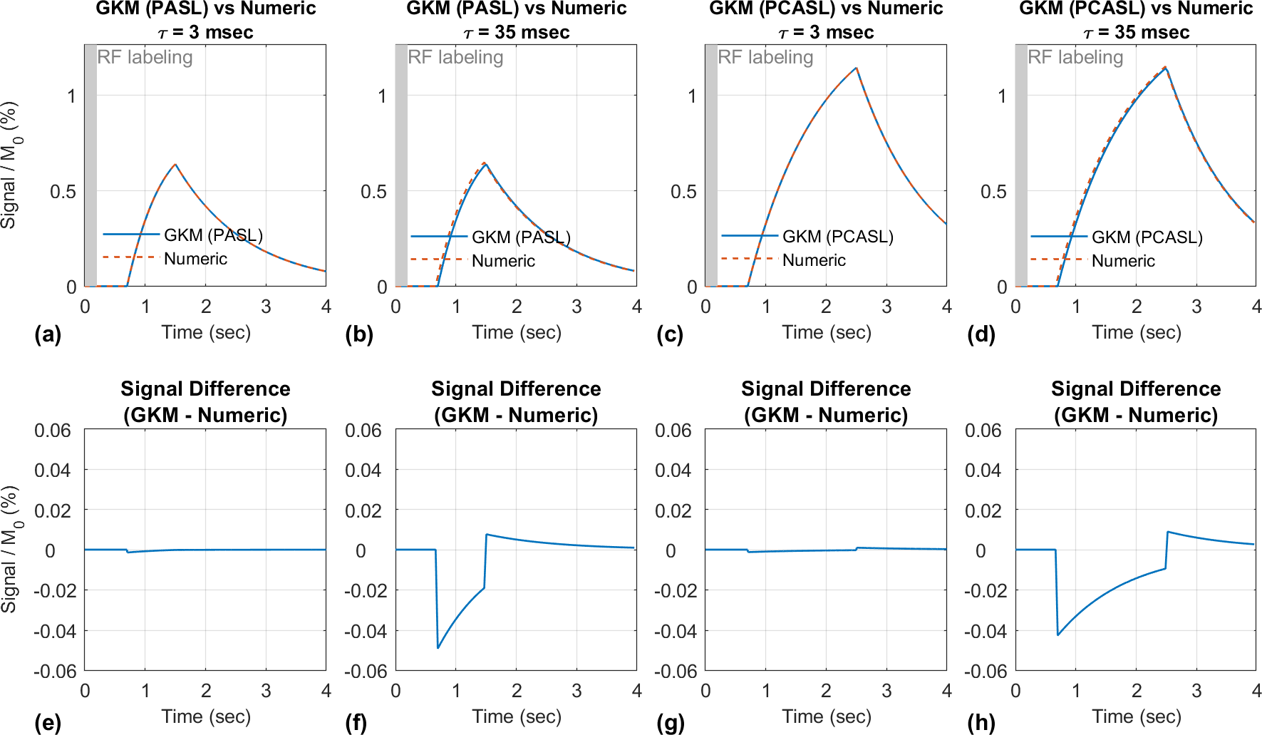
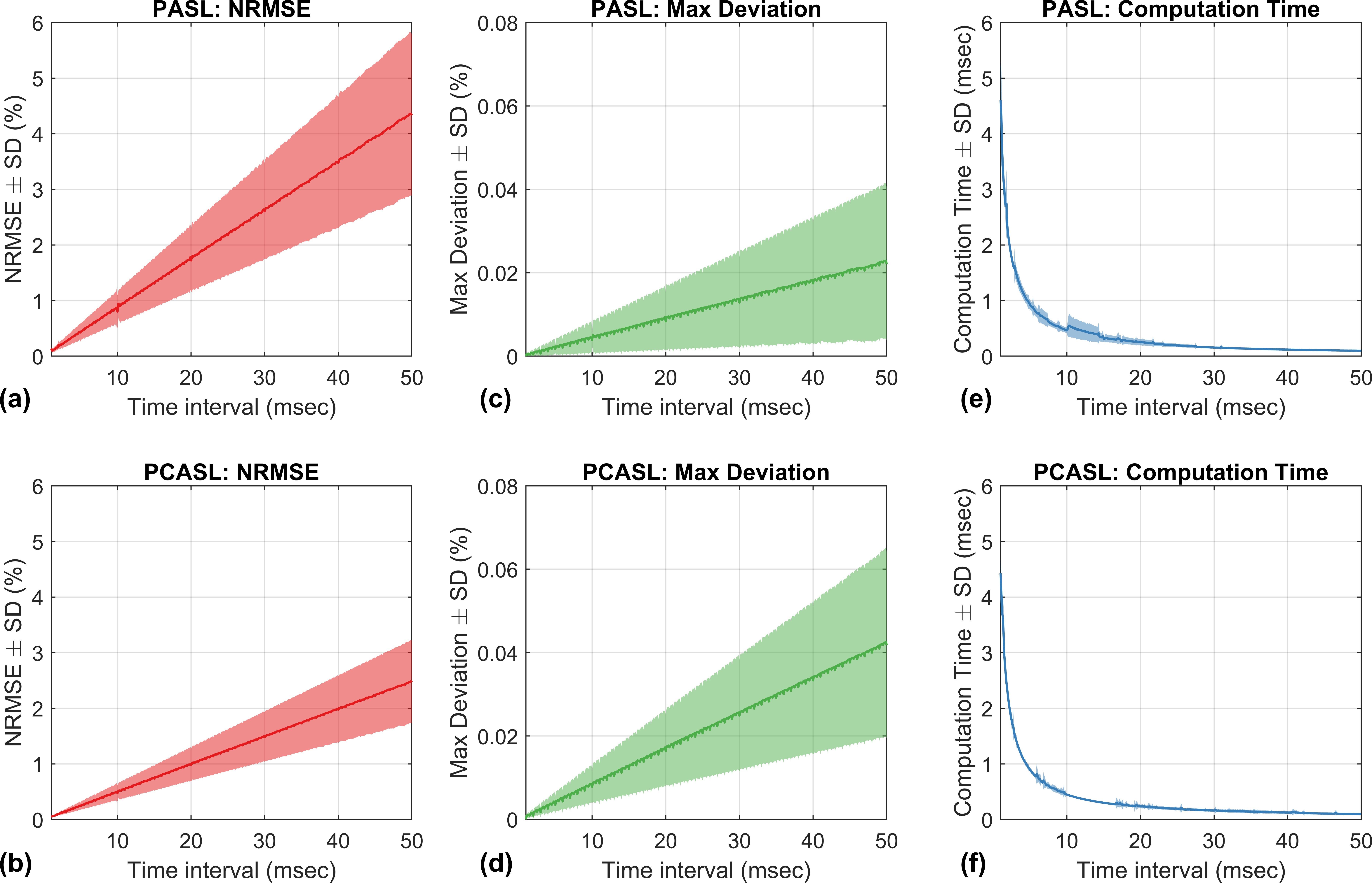
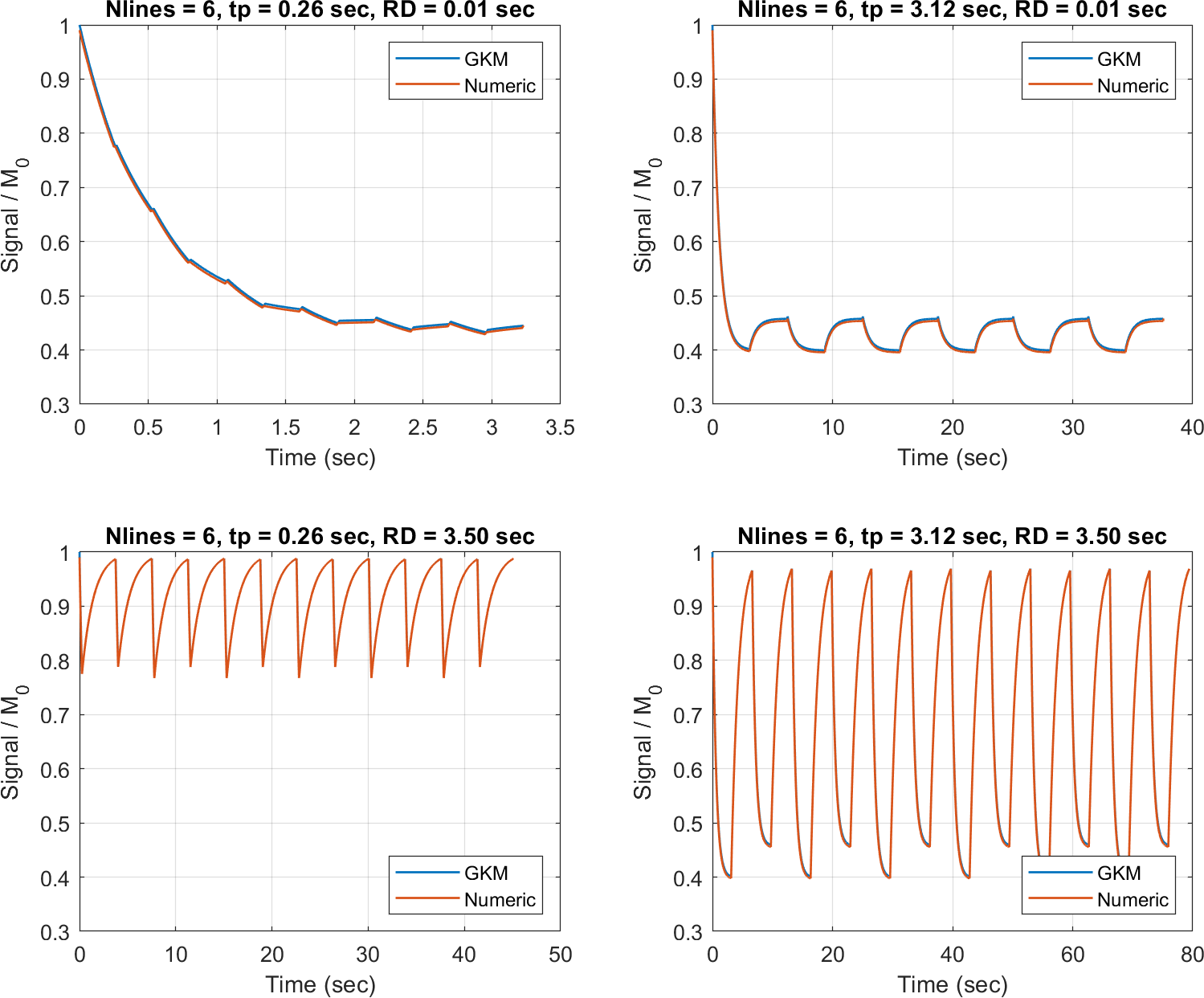
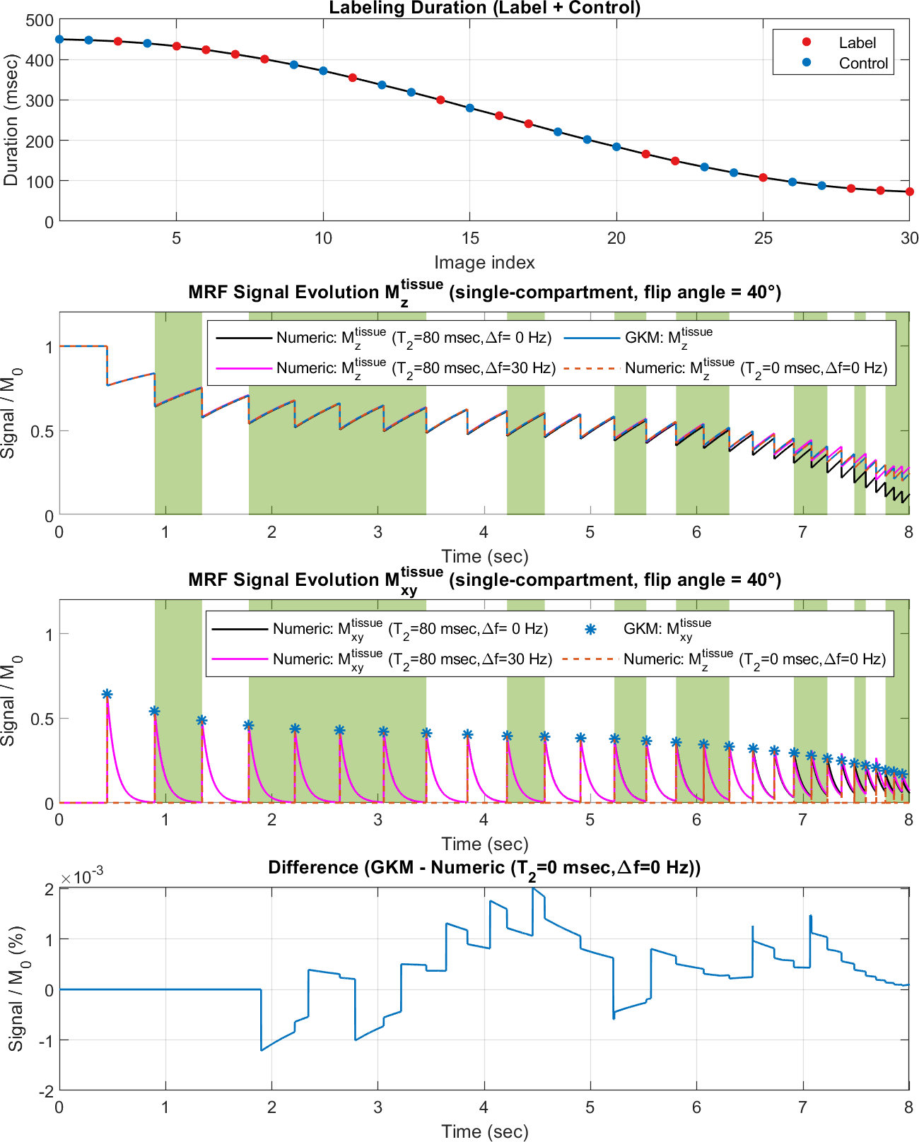
Figure 2 compares PASL and PCASL signals obtained with GKM and the numeric approximation using fixed time intervals of 3 and 35 ms. For time intervals of 3 and 35 ms, the maximum deviation between GKM and the numeric approximation was 0.002% and 0.07% for PASL, and 0.002% and 0.06% for PCASL, respectively. Figure 3 shows NRMSE, maximum deviation, and computation time as a function of the time interval (mean ± one SD) for PASL and PCASL. Figure 4 compares the theoretical signal evolutions for cine-ASL obtained with GKM and the numeric approximation (TR=$$$\tau$$$=10ms). This example demonstrates the numeric approximation can model the effects of flow under imaging RF pulses. Figure 5 compares the MRF-ASL signal evolutions obtained with GKM and the numeric approximation ($$$\tau$$$=1ms): the proposed method shows excellent agreement with GKM with a maximum signal difference of 0.002%. The proposed method deviates from GKM for TR $$$\cong$$$T2 (T2 = 80ms) when T2 effects and off-resonance are modeled.Discussion/Conclusion
We have demonstrated a numerical approximation to the GKM for ASL quantification. We have also characterized the tradeoff between accuracy and computation time through the selection of the timing interval. This numeric approximation is validated against GKM for PASL, PCASL, and nonconventional ASL pulse sequences. The numerical approach provides an excellent approximation to GKM as long as the time interval is sufficiently small. The proposed approach will enable quantification of transient-state ASL and ASL with irregular timing of RF labeling and/or severe off-resonance which are challenging for current techniques.Acknowledgements
We gratefully acknowledge funding support from NIH R01-HL130494.References
1. Buxton RB, Frank LR, Wong EC, Siewert B, Warach S, Edelman RR. A general kinetic model for quantitative perfusion imaging with arterial spin labeling. Magn. Reson. Med. 1998 doi:10.1002/mrm.1910400308.
2. Sled JG, Pike GB. Quantitative Interpretation of Magnetization Transfer in Spoiled Gradient Echo MRISequences. 2000;36:24–36 doi: 10.1006/jmre.2000.2059.
3. Graham SJ, Henkelman RM. Understanding pulsed magnetization transfer. J. Magn. Reson. Imaging1997 doi:10.1002/jmri.1880070520.
4. Jaynes ET. Matrix treatment of nuclear induction. Phys. Rev. 1955;98:1099–1105 doi:10.1103/PhysRev.98.1099.
5. Williams DS, Detre JA, Leigh JS, Koretsky AP. Magnetic resonance imaging of perfusion using spin inversion of arterial water. Proc. Natl. Acad. Sci. U. S. A. 1992;89:212–6.
6. Detre JA, Leigh JS, Williams DS, Koretsky AP. Perfusion imaging. Magn. Reson. Med.1992;23:37–45doi: 10.1002/mrm.1910230106
7. McConnell HM. Reaction rates by nuclear magnetic resonance. J. Chem. Phys. 1958;28:430–431 doi:10.1063/1.1744152.
8. Zaiss M, Zu Z, Xu J, et al. A combined analytical solution for chemical exchange saturation transfer and semi-solid magnetization transfer. NMR Biomed. 2015;28:217–230 doi: 10.1002/nbm.3237.
9. Woessner DE, Zhang S, Merritt ME, Sherry AD. Numerical solution of the Bloch equations provides insights into the optimum design of PARACEST agents for MRI. Magn. Reson. Med. 2005;53:790–799 doi:10.1002/mrm.20408.
10. A. C. Silva, W. Zhang, D. S. Williams, A. P. Koretsky, Estimation of water extraction fractions in rat brain using magnetic resonance measurement of perfusion with arterial spin labeling. Magn. Reson. Med.35, 58-68 (1997).
11. Bauer WR, Hiller KH, Roder F, Rommel E, Ertl G, Haase A. Magnetizationexchange in capillaries by microcirculation affects diffusion controlled spin-relaxation: a model which describes the effect of perfusion on relaxation enhancement by intravascular contrast agents. Magn Reson Med 1996;35:43–55.
12. Gloor M, Scheffler K, Bieri O. Quantitative magnetization transfer imaging using balanced SSFP. Magn Reson Med 2008;60:691–700.
13. Alsop DC, Detre JA, Golay X, et al. Recommended implementation of arterial spin-labeled perfusion MRI for clinical applications: A consensus of the ISMRM perfusion study group and the European consortium for ASL in dementia. Magn. Reson. Med. 2015;73:102–16 doi: 10.1002/mrm.25197
14. Troalen T, Capron T, Cozzone PJ, Bernard M, Kober F. Cine-ASL: A steady-pulsed arterial spin labeling method for myocardial perfusion mapping in mice. Part I. Experimental study. Magn. Reson. Med.2013;70:1389–1398 doi: 10.1002/mrm.24565.
15. Capron T, Troalen T, Cozzone PJ, Bernard M, Kober F. Cine-ASL: A steady-pulsed arterial spin labeling method for myocardial perfusion mapping in mice. Part II. Theoretical model and sensitivity optimization. Magn. Reson. Med. 2013;70:1399–1408 doi: 10.1002/mrm.24588.
16. Xu J, Qin Q, Wu D, et al. Steady pulsed imaging and labelingscheme for noninvasive perfusion imaging. Magn Reson Med.2016;75:238-248.
17. Su P, Mao D, Liu P, Li Y, Pinho MC, Welch BG, et al. Multiparametric estimation of brain hemodynamics with MR fingerprinting ASL. Magn Reson Med 2017;78:1812–23.
Figures
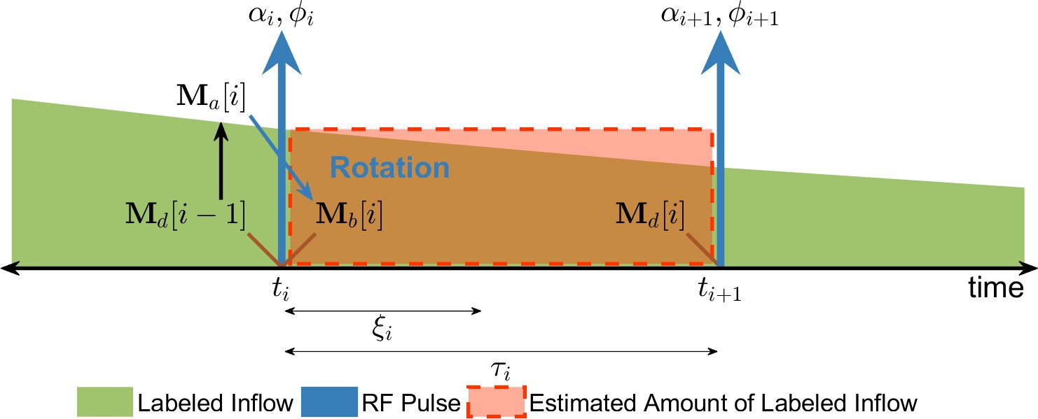
Figure 1. Illustration of the Bloch simulation with flow effects. The T1 decay of labeled arterial blood (green) over each interval is exaggerated. The symbols αi/φi/ti/ξi/τi indicate flip angle/phase/start time/measurement time/duration for the ith time interval. Using piecewise constant approximation, the actual amount of labeled blood over the time interval of duration $$$\tau_i$$$ (green) is estimated by the area of a rectangle (dashed red box). During each interval, tissue magnetization relaxes with a new pseudo M0 term: M0+s(ti)·T1app.