3257
QSM streaking suppression with L1 data fidelity terms
Carlos Milovic1,2,3, Mathias Lambert1,2,3, Christian Langkammer4, Kristian Bredies5, Cristian Tejos1,2,3, and Pablo Irarrazaval1,2,3
1Department of Electrical Engineering, Pontificia Universidad Catolica de Chile, Santiago, Chile, 2Biomedical Imaging Center, Pontificia Universidad Catolica de Chile, Santiago, Chile, 3Millennium Nucleus for Cardiovascular Magnetic Resonance, Santiago, Chile, 4Department of Neurology, Medical University of Graz, Graz, Austria, 5Institute of Mathematics and Scientific Computing, University of Graz, Graz, Austria
1Department of Electrical Engineering, Pontificia Universidad Catolica de Chile, Santiago, Chile, 2Biomedical Imaging Center, Pontificia Universidad Catolica de Chile, Santiago, Chile, 3Millennium Nucleus for Cardiovascular Magnetic Resonance, Santiago, Chile, 4Department of Neurology, Medical University of Graz, Graz, Austria, 5Institute of Mathematics and Scientific Computing, University of Graz, Graz, Austria
Synopsis
L2-norm based data fidelity terms in QSM functionals account for Gaussian noise in the phase or complex domain. These approaches are not robust against phase inconsistencies, such as artifacts from previous steps, intra-voxel dephasing, etc. To deal with these errors and to suppress streaking artifacts we present L1-norm algorithms that correct for salt-and-pepper noise. We use simulations and in-vivo acquisitions to show their streaking suppression capabilities. Furthermore, L1 methods do not require magnitude information, and they were able to achieve similar results without ROI masks. This may facilitate susceptibility studies of cortical areas and regions outside the brain.
PURPOSE
Estimating the susceptibility of tissues is an ill-posed inverse problem, prone to noise amplification and artifact generation1,2. The most prominent artifact is the so-called streaking artifact. Phase inconsistencies to the expected magnetization field are projected along the magic cone in the deconvolution process. Traditionally, streaking artifacts are reduced using regularizers, at the expenses of losing image sharpness or details3-5. Modifications to the data fidelity term to account for more realistic noise models have been able to further reduce the impact of streaking artifacts, especially those arising from regions with low MR signal6-8. Unfortunately, these models require accurate signal magnitude representations, and masks that rejects erroneous phase data. This is often a complex task that may lead to the loss of cortical areas due to size reduction of the region of support (erosion of the tissue mask). Here we present two new data fidelity terms that model salt-and-pepper noise to account for phase inconsistencies and prevent streaking, one in the (linear) phase domain, and the other in the (nonlinear) complex image domain.METHODS
In a Bayesian approach, the nonlinear QSM method models Gaussian noise in the complex image domain6-8. A magnitude-weighted linear data fidelity term may be interpreted as a first-order approximation8. In this work, we compare the traditional linear and nonlinear L2-norm models with two L1-norm alternatives: $$$argmin_{\chi }\frac{1}{2}\|W\left(F^{H}DF\chi-\varphi\right)\|_1+TV(\chi)$$$ and $$$argmin_{\chi }\frac{1}{2}\|W\left(e^{iF^{H}DF\chi}-e^{i\varphi}\right)\|_1+TV(\chi)$$$, where W is a magnitude-based weight or ROI mask, D is the frequency dipole kernel, F the Fourier transform with FH its inverse, Φ the input local phase and χ the susceptibility distribution. For simplicity, we use TV as the regularization. To reduce computational processing time, we solved these optimization problems using ADMM. To decouple the linear data fidelity term, an auxiliary variable $$$z=F^HDF\chi-\varphi$$$ is needed. For the nonlinear data fidelity term, two additional auxiliary variables $$$z_1=F^HDF\chi$$$ and $$$z_2=e^{iz_1}-e^{i\varphi}$$$ are needed. Then, the z, z1, z2, and χ subproblems are solved in a similar way as in Bilgic9 and Milovic8,10, using a proximal operation for z and z2. We use internal Newton-Raphson iterations to solve z1.These solvers were compared using forward simulations from a COSMOS (complex noise, SNR=100) reconstruction (QSM Challenge 1.0 dataset11) with different W weights (no ROI mask, ROI masks, and SNR weights). We also used one simulated acquisition from the QSM Challenge 2.0 dataset12. We used the provided frequency map from the Sim2SNR2 data as input, due to its high noise level and intra-voxel dephasing effects. In vivo reconstructions are also provided, using the QSM Challenge 1.0 dataset.
RESULTS
Figure 1 presents different reconstructions varying the ROI mask (with and without) and introducing magnitude weights (W). Regularization parameter was obtained optimizing RMSE (Table 1). Notably, L1 reconstructions without masks or magnitude information were possible, with similar visual results to those masked. Without phase inconsistencies inside the ROI, L2-norm methods achieved better metric scores. Figure 2 and Table 2 show the results of reconstructing the Challenge 2.0 dataset. L1 reconstructions achieved lower errors for all metrics. Nonlinear reconstructions performed slightly better than their linear counterparts. In vivo reconstructions (Figure 3) show less streaking from the venous system and more structural details -especially at cortical regions- for the L1 methods.DISCUSSION & CONCLUSION
Despite having slightly worse global metrics in the first experiment (RMSE and SSIM, Challenge 1.0), L1 reconstructions seemed to be more robust against phase noise, producing sharper images. Irrespective of the data fidelity weight or the mask used, L1 methods produced optimal reconstructions with similar associated regularization weights, within one order of magnitude. L2-norm methods had optimal regularization weights depending on the mask or weight in a range larger than two orders of magnitude. This makes parameter fine-tuning easier for L1-norm methods. L1 reconstructions were also more robust to phase errors, making the ROI masking process less relevant. This may allow QSM algorithms to better explore cortical areas and may facilitate reconstructions of regions outside the brain. It also prevents streaking from strong intra-voxel dephasing effects, as seen in the Challenge 2.0 dataset, where L1 reconstructions performed significantly better and were more robust to noise at the venous system. The nonlinear L1 method seemed to produce smoother results than the linear method, without loss of information.Acknowledgements
Fondecyt 1191710, Anillo 190064, Millennium Nucleus for Cardiovascular Magnetic ResonanceReferences
1. Wharton CMRB 2005. 2. Shmueli MRM 2009. 3. de Rochefort MRM 2008. 4. Kressler IEE-TMI 2010. 5. Liu MRM 2011. 6. Liu MRM 2013. 7. Wang IEE-TBE 2013. 8. Milovic MRM 2018a. 9. Bilgic SPIE 2015. 10. Milovic MRM 2018b. 11. Langkammer MRM 2018. 12. Marques ISMRM 2019.Figures

Figure 1. Reconstructions of the COSMOS-based forward simulations, optimizing RMSE. Nonlinear L2-norm results not displayed. Each row corresponds to different data fidelity spatially variable weights (W=1, W=Mask, and W=Magnitude). For comparison reconstructions without a mask (W=1) are displayed in the last row, but using the optimal parameters for W=mask.

Figure 2. Optimal (RMSE) reconstructions using linear and nonlinear algorithms with L1-norm and L2-norm terms. Each result shows a global view (top) and a zoomed-in view centered at the calcification (bottom).
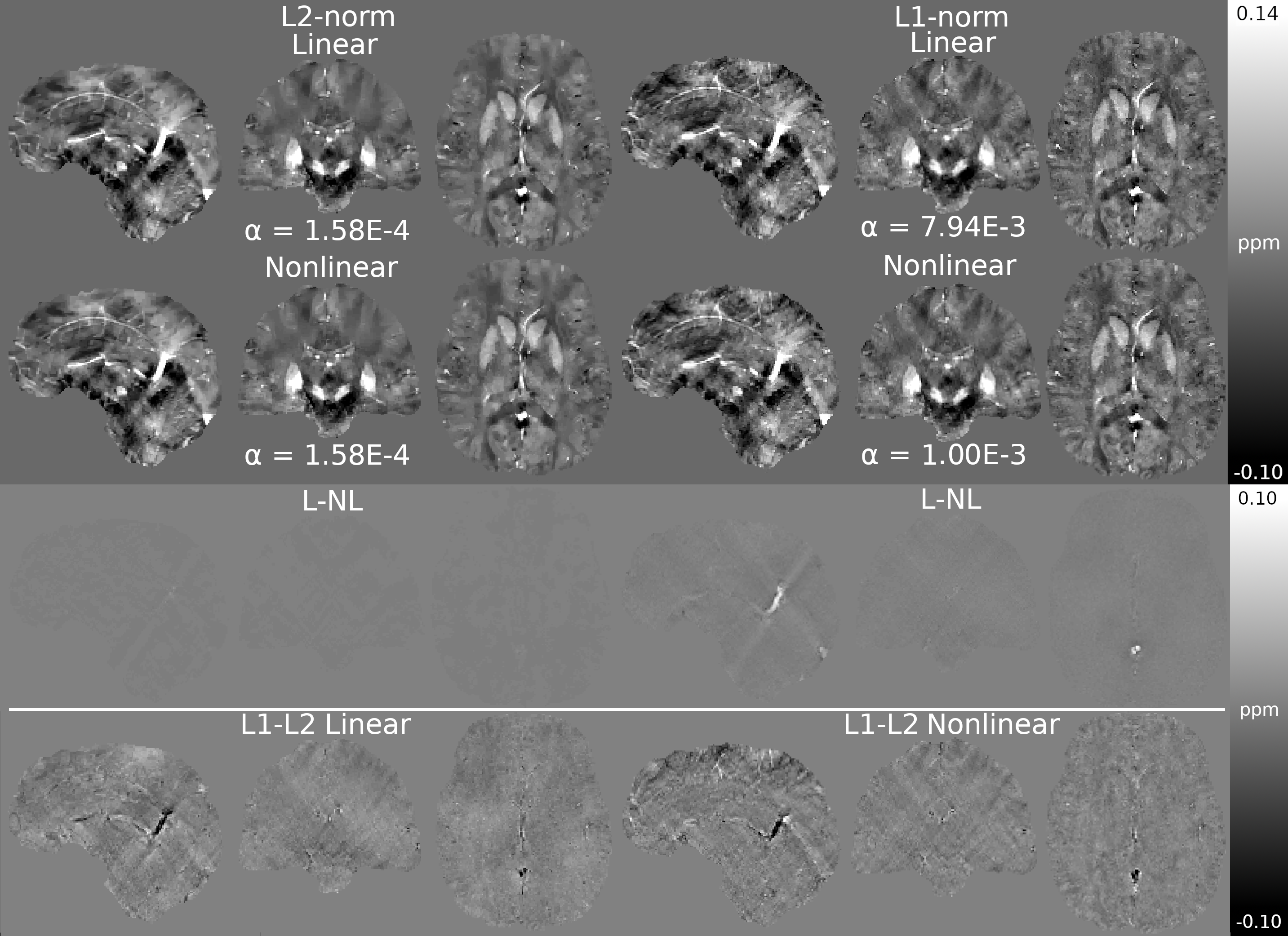
Figure 3. In vivo results (top) and difference maps (bottom).
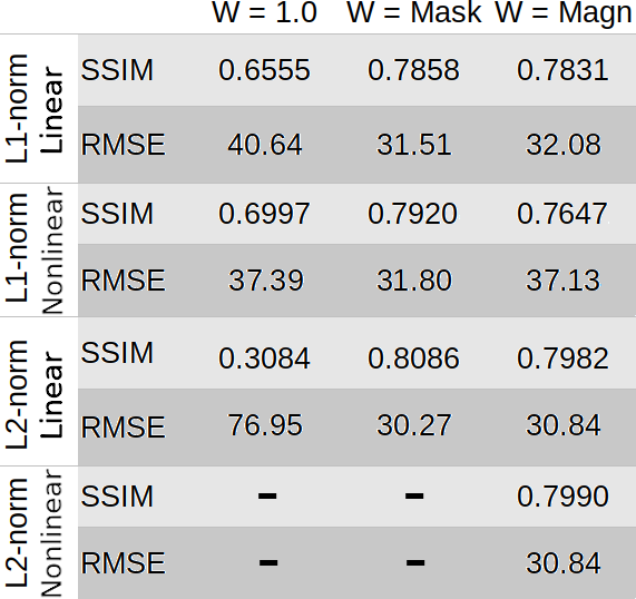
Table 1. RMSE and SSIM scores for the COSMOS-based simulations.
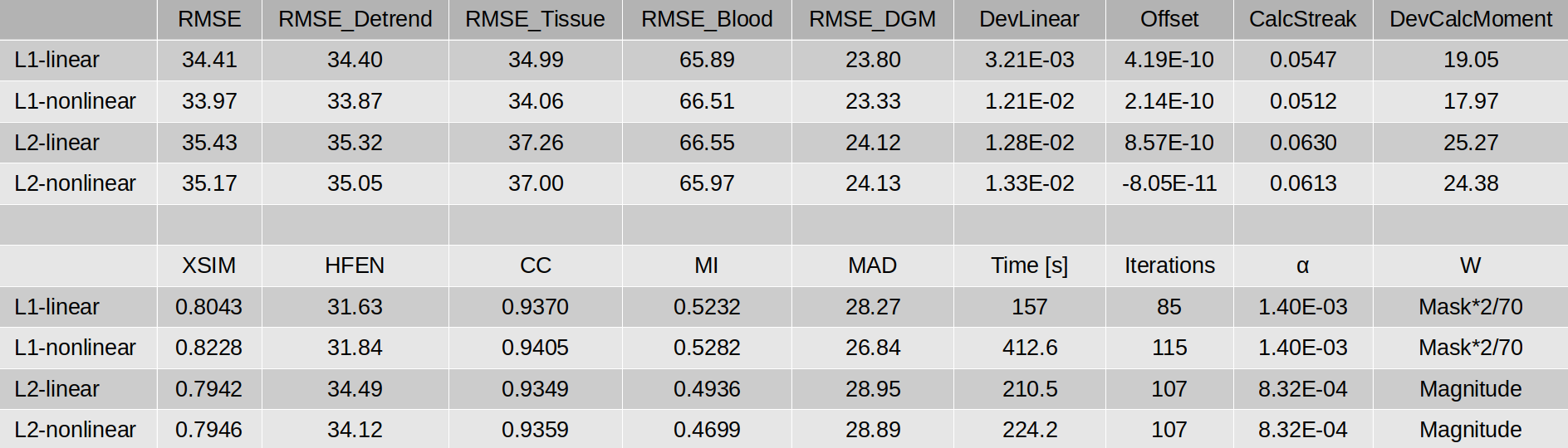
Table 2. Error metric scores for reconstructions of the Challenge 2.0 SIM2SNR1 data.