Introduction

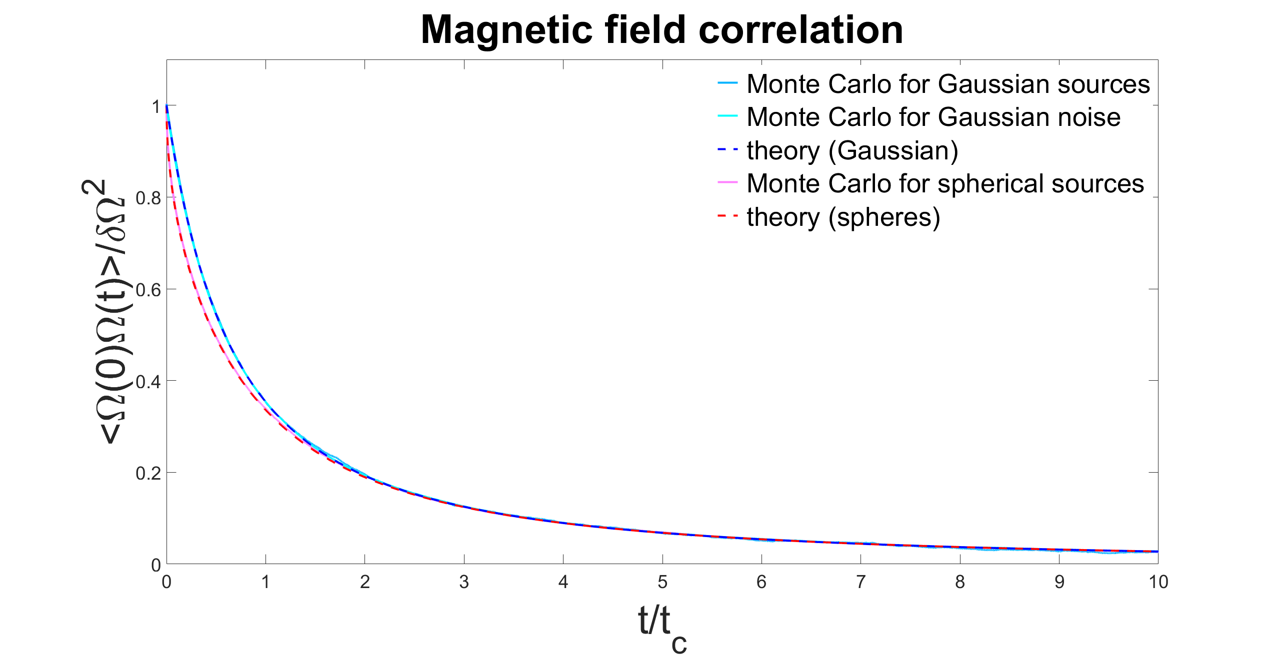
The magnetic susceptibility of tissue microstructure produces characteristic signatures in R2* decay$$$^{1-7}$$$. These arise from variations in the magnetic field experienced by water molecules as they diffuse around microstructural sources of magnetic susceptibility. The correlation time $$$t_c=l_c^2/D$$$ associated with these variations is the interval required for spins to diffuse a distance equal to the characteristic length scale $$$l_c$$$ of the microstructure, where $$$D$$$ is the diffusion coefficient. For times much shorter than $$$t_c$$$, the spins are in the static dephasing regime and the logarithm of the signal exhibits a quadratic dependence on time. At times much longer than $$$t_c$$$, the spins are in the diffusion narrowing regime and the signal decay becomes asymptotically monoexponential. The transition between these two regimes can, in principle, be used to extract $$$t_c$$$, which in turn determines $$$l_c$$$.

In the weak field approximation$$$^{2-8}$$$ the signal decay is expressed as a cumulant expansion and truncated after the quadratic term $$S\left(t\right)=S_0e^{-R_2t}\left\langle e^{i\phi\left(t\right)}\right\rangle\approx{S_0}e^{-R_2t-\left\langle\phi^2\left(t\right)\right\rangle/2}\;\;\;\;\left[1\right]$$ where $$\phi\left(t\right)=\int_0^t\mathrm{d}t_1\,\Omega\left(t_1\right) \;\;\;\;\left[2\right]$$ is the cumulative phase of the spins and $$$\Omega\left(t\right)=\gamma{B_0}\left(t\right)$$$ is their Larmor frequency. The phase variance $$\left\langle\phi^2\left(t\right)\right\rangle=\int_0^t\mathrm{d}t_1\int_0^t\mathrm{d}t_2\,\left\langle\Omega\left(t_1\right) \Omega\left(t_2\right)\right\rangle\;\;\;\;\left[3\right]$$ is fully described by the temporal magnetic field correlation$$$^7$$$, which can be calculated analytically for certain geometries, notably a random distribution of permeable Gaussian sources of magnetic susceptibility, each with susceptibility profile $$$\chi\left(\mathbf{r}\right)=\chi_0e^{-\left|\mathbf{r}\right|^2/2l_c^2}$$$. The magnetic field correlation in this case equals $$\left\langle\Omega\left(0\right) \Omega\left(t\right)\right\rangle=\frac{\delta\Omega^2}{\left(1+t/t_c\right)^{3/2}}\;\;\;\;\left[4\right]$$ Similarly, for a random distribution of permeable spheres$$$^8$$$, each with susceptibility $$$\chi\left(\mathbf{r}\right)=\chi_0$$$ and radius $$$R=\left(6\sqrt{\pi}\right)^{1/3}l_c$$$, the magnetic field correlation equals $$\left\langle\Omega\left(0\right) \Omega\left(t\right)\right\rangle=\delta\Omega^2 \left[\mathrm{erf}\left(\sqrt{\frac{t_c}{t}}\right)+\frac{2}{\sqrt{\pi}}\left(\frac{t}{t_c}\right)^{3/2}\left(1-e^{-t_c/t}\right)+\frac{1}{\sqrt{\pi}}\left(\frac{t}{t_c}\right)^{1/2}\left(e^{-t_c/t}-3\right)\right]\;\;\;\;\left[5\right]$$ Here $$$\delta\Omega^2$$$ is the variance in Larmor frequency due to magnetic field inhomogeneity. The order of the cumulants is reflected in the power of the dimensionless parameter $$$\alpha=\delta\Omega\,t_c$$$, which represents the dephasing due to field inhomogeneity over the time interval $$$t_c$$$. Thus the weak field approximation is assumed to be valid in the limit $$$\alpha\ll1$$$.

In this work, we simulate the motion of water molecules among susceptibility sources of various geometries, and calculate the magnetic field correlation and signal decay over a range of $$$\alpha$$$. The results are validated against theory, and used to examine the regime of validity of the weak field approximation.

Methods

Monte Carlo simulations were performed by modeling the free diffusion of water through a magnetic field perturbed by randomly distributed Gaussian and spherical sources of magnetic susceptibility with volume fraction 0.1. A magnetic field consisting of spatially correlated Gaussian-distributed noise was also considered. This is of interest because the magnetic field correlation is identical to that in equation [4], but the higher order cumulants are also evaluable.

The cumulative phase $$$\phi\left(t_i\right)$$$ of each random walker at each time point $$$t_i$$$ was calculated and stored. Since the phases varied linearly with $$$\delta\Omega$$$, they could be arbitrarily scaled after the simulation, and the signal dephasing $$$\left\langle e^{i\phi\left(t_i\right)}\right\rangle$$$ reevaluated.

Results

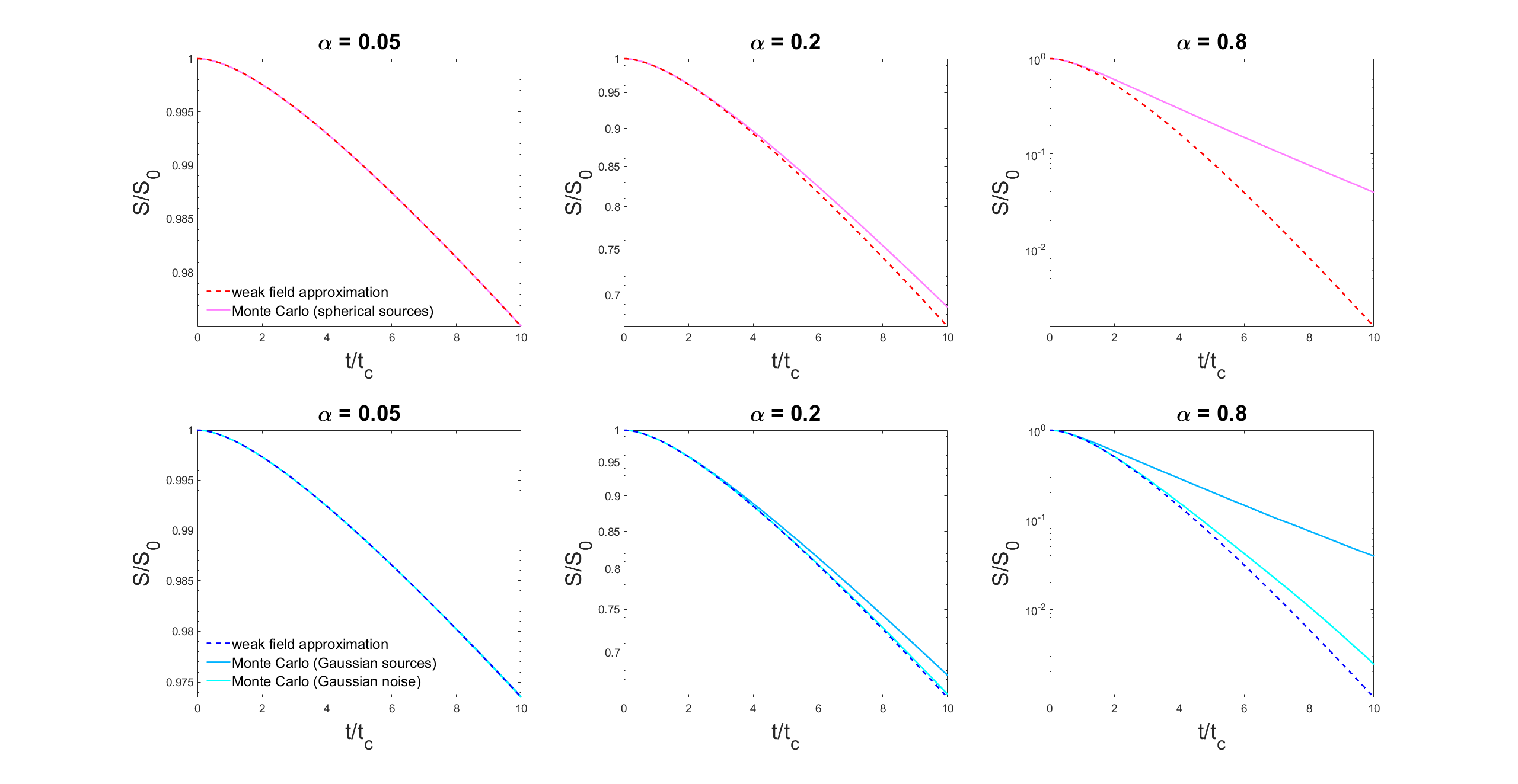
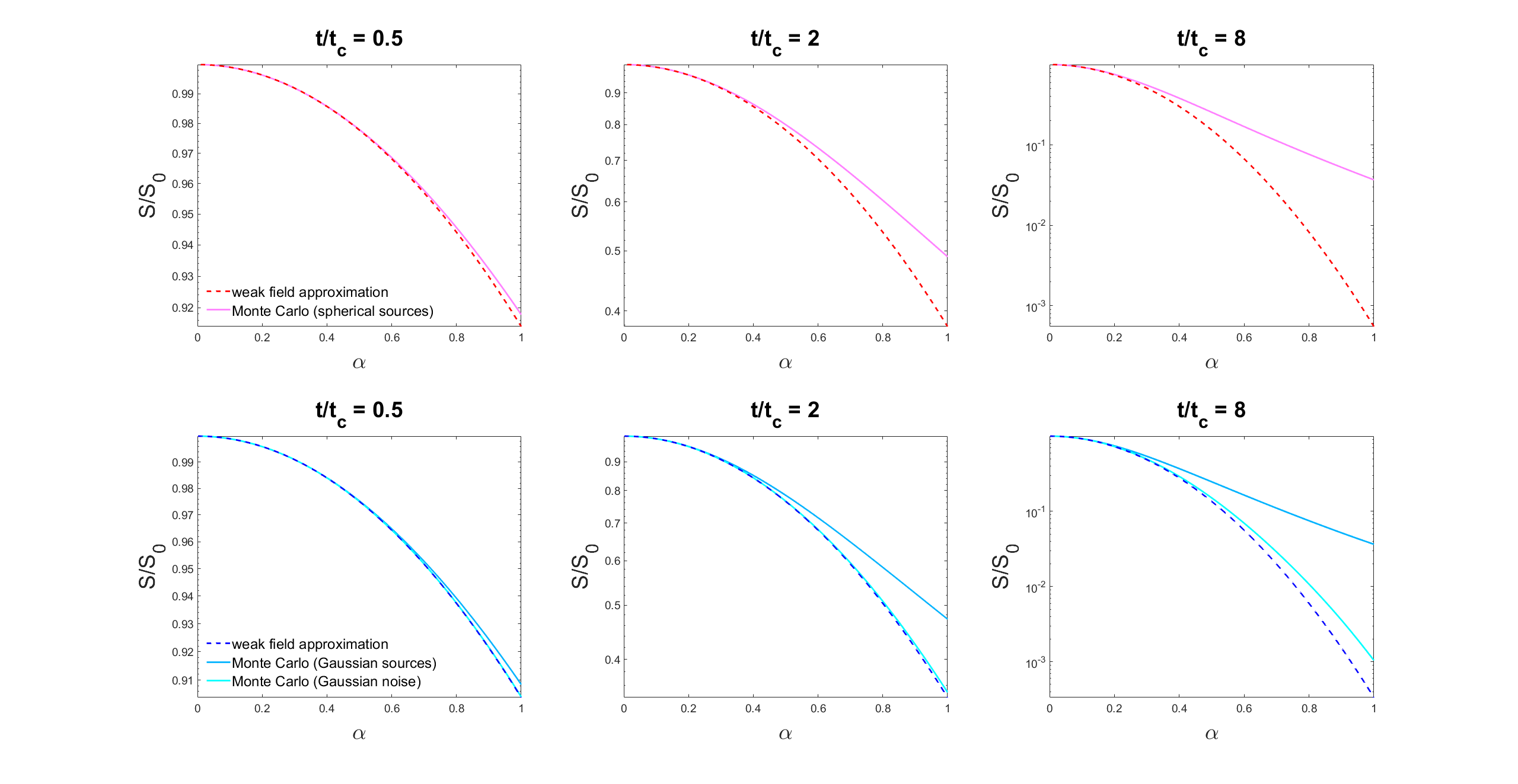
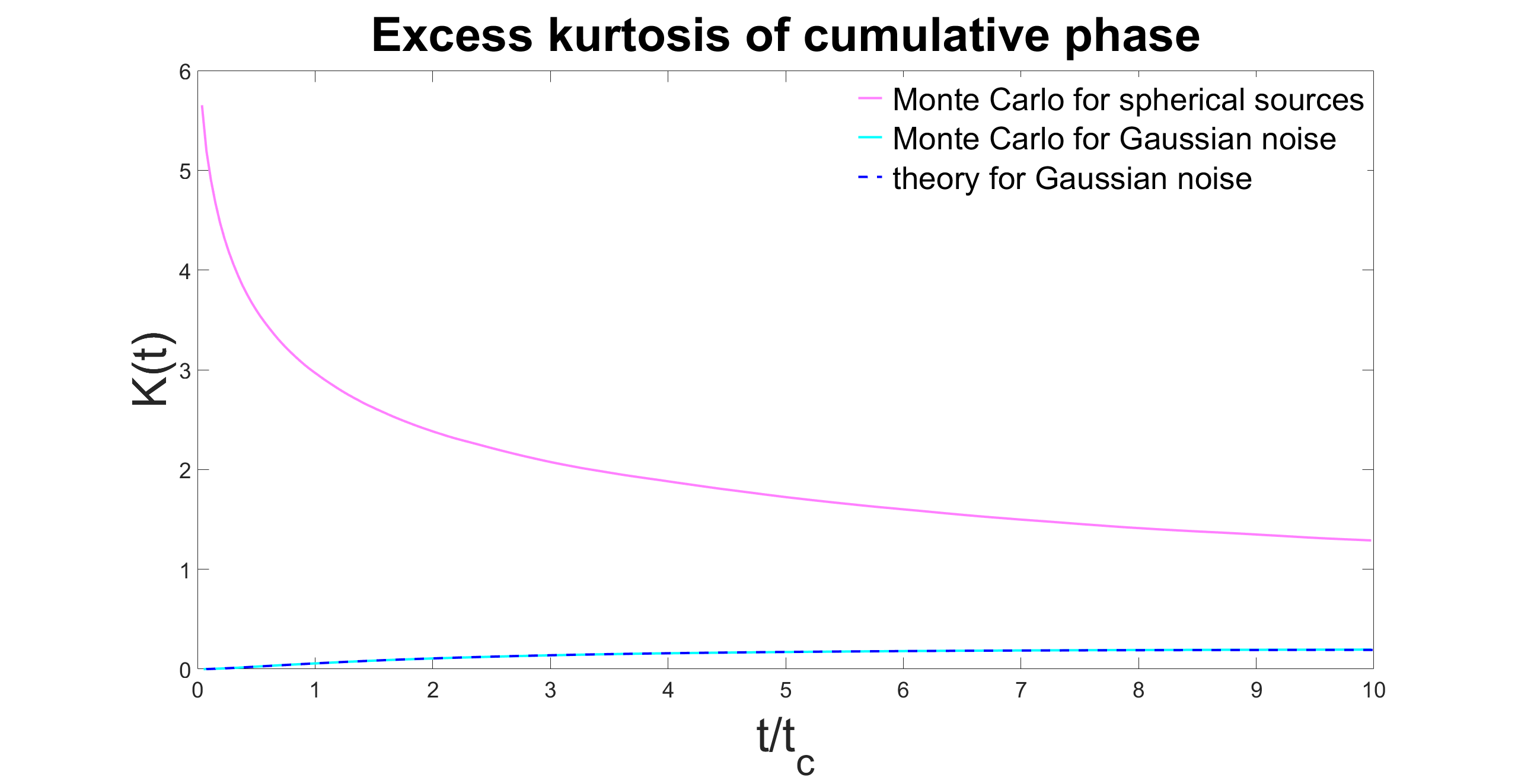
The magnetic field correlation as evaluated from Monte Carlo simulations agreed well with theory for all geometries (Figure 1). Note that $$$\left\langle\Omega\left(0\right) \Omega\left(t\right)\right\rangle$$$ is lower for spherical sources than Gaussian sources at short $$$t$$$, presumably due to the discontinuity of the magnetic field at the sphere surface. However, the signal $$$\left\langle e^{i\phi\left(t\right)}\right\rangle$$$ evaluated from Monte Carlo simulations deviated from the weak field approximation for both large $$$\alpha$$$ and long times $$$t/t_c$$$ (Figures 2 and 3). This discrepancy demonstrates the importance of higher order terms in the cumulant expansion. The fourth order cumulant equals $$$K\left(t\right)\cdot\left\langle\phi^2\left(t\right)\right\rangle^2$$$ where $$$K\left(t\right)$$$ is the excess kurtosis of the cumulative phase $$K\left(t\right)=\frac{\left\langle\phi^4\left(t\right)\right\rangle}{\left\langle\phi^2\left(t\right)\right\rangle^2}-3\;\;\;\;\left[6\right]$$
This is displayed in Figure 4. Note that the kurtosis of the cumulative phase approaches that of the underlying magnetic field as $$$t\rightarrow{0}$$$ since $$\lim_{\delta{t}\rightarrow{0}}\phi\left(\delta{t}\right)=\gamma{B_0}\left(0\right)\delta{t}\;\;\;\;\left[7\right]$$ It follows that $$$K\left(0\right)=0$$$ for spins diffusing through a magnetic field consisting of spatially correlated Gaussian-distributed noise.

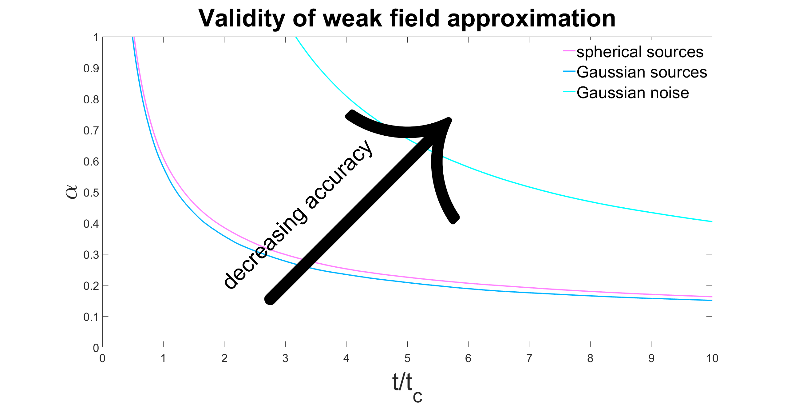
The regime of validity of the weak field approximation is plotted as a function of $$$\alpha$$$ and $$$t/t_c$$$ in Figure 5. The weak field limit may be characterized by the condition that the fourth-order cumulant be much smaller than the second-order cumulant. For the geometries considered here, the kurtosis of the cumulative phase is $$$K\left(t\right)\sim{1}$$$, from which it follows that the weak field limit may most simply be characterized by the condition that the variance of the cumulative phase be small, $$$\left\langle\phi^2\left(t\right)\right\rangle\ll{1}$$$.

Discussion

In reality, the sources of magnetic susceptibility may be nonoverlapping, in which case their distribution is not truly random. This can be taken into account by incorporating the autocorrelation function of a distribution of randomly packed spheres$$$^9$$$ into the calculation of $$$\left\langle\Omega\left(0\right)\Omega\left(t\right)\right\rangle$$$. The result is slightly lower than that of a purely random distribution over all $$$t$$$, reflecting the higher degree of ordering. For sources that are impermeable to water, no theory exists except in the limit of low volume fraction$$$^6$$$. However, Monte Carlo simulations demonstrate that this too has a small effect on the magnetic field correlation, reflecting the exclusion of the field inside the sources and the hindered diffusion of water around the sources. Neither of these considerations qualitatively affects the regime of validity of the weak field approximation.

Conclusions

We have demonstrated that the R2* decay rate deviates from that predicted by the weak field approximation at long times $$$t\gg{t_c}$$$, even for $$$\delta\Omega\,t_c\ll{1}$$$. Therefore, the weak field limit is better described by the condition $$$\left\langle\phi^2\left(t\right)\right\rangle\ll{1}$$$.

Acknowledgements

P.S. is grateful to Sze Tan, PhD, for valuable discussions. This work was supported in part by NIH grants NIH NS039135 and P41 EB017183.