3246
Shearlet-based susceptibility map reconstruction with iterative reweighting and nonlinear data fitting1German Cancer Research Center (DKFZ), Heidelberg, Germany, 2Faculty of Physics and Astronomy, Heidelberg University, Heidelberg, Germany
Synopsis
The QSM algorithms tested in the 2016 Reconstruction Challenge showed oversmoothing effects and a notable loss of details. A multicale shearlet system was used to reconstruct the susceptibility map. Iterative reweighting of the coefficients led to a sparse image in the shearlet space. The result shows that shearlets are useful to obtain quantitative susceptibility maps which are rich in detail and simultaneously can achieve a top ten result in the ranking of the 2016 Reconstruction Challenge.
Introduction
Many of the susceptibility maps presented in the 2016 QSM Reconstruction Challenge [1] were poor in detail because the reconstructions were characterized by oversmoothing. The purpose of this work is to show the usefulness of a shearlet-based reconstruction to obtain detailed susceptibility maps within a top ten ranking relative to the applied classical image quality measures of the 2016 Challenge.Theory
Quantitative susceptibility mapping (QSM) is the attempt to map the tissue magnetic susceptibility. The following inverse problem is solved in the Fourier domain:$$ \psi (\textbf{k}) = D(\textbf{k}) \chi (\textbf{k}) , \quad \textbf{k} = (k_x,k_y,k_z) \in \mathbb{R}^3, \quad (1) $$
$$$\psi$$$ denotes the measured phase data, $$$\chi$$$ is the tissue magnetic susceptibility to be determined and $$$D$$$ denotes the dipole kernel:
$$ D(\textbf{k}) := \frac{1}{3}- \frac{k_z^2}{|\textbf{k}|^2}. $$
Equation (1) is ill-posed due to $$$D(\textbf{k}) = 0$$$ at the zero cone $$$\Gamma_0$$$,
$$\Gamma_0=\lbrace \textbf{k} \in \mathbb{R}^3 | k_x^2+k_y^2-2k_z^2 = 0 \rbrace.$$
Hence, prior knowledge must be used to achieve a unique solution.
The sparsity of MR images after applying a multilevel transform, e.g. a shearlet transform $$$\Psi$$$ is used as a prior.
Suppose $$$\chi^*$$$ is the true susceptibility, $$$y$$$ the measured phase and $$$E=\mathcal{F}^{-1}D\mathcal{F} $$$ is the forward operator with $$$\mathcal{F}$$$ denoting the Fourier transform. Then the minimization problem
$$ \underset{\chi}{min} ||W\Psi \chi||_1 + \frac{\beta}{2}||y-E\chi||_2^2 $$
with weights $$ W = \text{diag}(\sigma_1,...,\sigma_N) \quad \text{and} \quad \sigma_i = \begin{cases} \frac{1}{|\Psi \chi_i^*|}, \quad & \Psi x_i \neq 0, \\ \infty, \quad & otherwise,\end{cases} $$
will find sparser solutions than the unweighted minimization problem [2].
Since the true solution is not available, one considers a sequence of weights
$$ \sigma_i^k = \frac{1}{|(\Psi \chi^k)_i|+ \epsilon}, $$
where $$$\epsilon > 0$$$ is small and $$$(x^k)_k \subset \mathbb{R}^N$$$ are approximations to the true susceptibility $$$\chi^*$$$. They are obtained by
$$\chi^k = \underset{\chi}{\text{argmin}}||W^{k-1}\Psi \chi||_1 + \frac{\beta}{2}||y-E\chi||_2^2 $$.
As the coefficients of a multiscale transform decrease with higher scales, the weighting matrix $$$W$$$ is given scalewise to avoid erroneous zero coefficients [3,4].
$$ W^j_{k+1}d^j = diag\left(\frac{\lambda_j^{k+1}}{|(\Psi x_{k+1})_j|+ \epsilon}\right)d^j, $$
where $$$\Psi x = \left(\Psi_j x\right)_{j=0,...,J} = \left(\langle \Psi_{j,l},x \rangle \right)_{j = 0,...,J,l=1,...,N_j},$$$ divides the shearlet coefficients into $$$J$$$ scales and $$$\lambda_j^{k+1} = \underset{l}{max} \left(\langle \Psi_{j,l},x_{k+1} \rangle \right)_l $$$ denotes the maximum of the shearlet coefficients of $$$x_{k+1}$$$ belonging to scale $$$j$$$.
Methods
To evaluate the algorithm it was applied to local phase data from the 2016 Reconstruction Challenge, that also provided two different ground truths and four error metrics [1]. Here, $$$\chi_{33}$$$ from the STI solution was used as ground truth. For visual comparison, an additional susceptibility map was computed with truncated k-space division (TKD) with a threshold of 0.2.The proposed algorithm consists of three steps. In Step 1 an iterative solver is used to compute an initial guess $$$\chi_0$$$ and a susceptibility map $$$\chi_{well}$$$ from the data in the well-conditioned region $$$(|D| > 0.2)$$$ [5]. The second step includes $$$\chi_{well}$$$ as a data-fit term [5] in the following problem: $$\underset{\chi}{min} ||\Psi \chi||_1 + ||M\chi-\chi_{well}||_2^2 \quad (2)$$ where $$$M = \mathcal{F}^{-1}R\mathcal{F}$$$ is a linear operator including the binary mask $$$R$$$ which defines the well-conditioned region and $$$\Psi$$$ is the shearlet transform [6]. Step 3 consists of an additional nonlinear data fit around the solution $$$\chi$$$ of Step 2: $$\underset{\tilde{\chi}}{\text{min}}||\cos(y)-\cos(E(\tilde{\chi}))||_2^2 + ||\sin(y)-\sin(E(\tilde{\chi}))||_2^2 + ||\tilde{\chi}-\chi||_2^2 \quad (3)$$. Equation (3) is solved by setting its gradient equal to zero and applying Newton's method.
In Step 2, the alternating direction method of multipliers (ADMM) is applied. This is an algorithm that solves convex optimization problems by subdividing them into smaller pieces, each of which are then easier to handle. Equation (2) is solved in three steps: $$ \begin{split} \chi_{k+1} &= \underset{\chi}{arg min} \: \frac{\beta}{2} || \chi_{well}- Mx||_2^2 + \frac{\mu}{2} ||d_k - \Psi \chi - b_k||_2^2 \quad (4) \\ d_{k+1} &= \underset{d}{arg min} \: ||d||_1 + \frac{\mu}{2} ||d - \Psi \chi_{k+1} - b_k||_2^2 \quad (5) \\ b_{k+1} &= b_k + \Psi \chi_{k+1} - d_{k+1}, \end{split} $$ for an additional parameter $$$\mu > 0$$$. The $$$\chi$$$-update is solved by setting the gradient of Equation (4) to zero and using an iterative solver. The solution of Equation (5) provides the shearlet coefficients. The iterative reweighting can be directly incorperated into this subproblem by replacing Equation (5) by $$ d_{k+1} = \underset{d}{arg min} \: ||W_{k+1}d||_1 + \frac{\mu}{2} ||d - \Psi \chi_{k+1} - b_k||_2^2 \quad (6)$$ Equation (6) is called the proximal step and is explicitly solved by shrinking: $$ d_{k+1} = \text{shrink}\left(\Psi \chi_{k+1} + b_k, \frac{1}{\mu}W \right),$$ where the shrinkage function $$\text{shrink}(u,\omega) = \begin{cases} max\left(||u||-\omega,0\right)\frac{u}{||u||}, \quad &u\neq 0\\ 0,\quad \quad &u = 0 \end{cases}$$ is applied element-wise. For this work the parameters were chosen to $$$\beta = $$$2.67*103 and $$$\mu =$$$2*105.
Results & Discussion
Figure 1 displays the susceptibility maps of the proposed algorithm. The classical image quality measures for the susceptibility maps of each step are shown in Table 1. As one can see in the second step, the parameters were choosen to reduce the root mean squared error (RMSE), accepting therefore an oversmoothed intermediate map. The last step removes the oversmoothing and produces a detailed susceptibility map with acceptable to very good image quality measure values (best ROI error).In Figure 2, susceptibility maps of the proposed method, the ground truth and TKD are shown.
Acknowledgements
This work was supported by a grant from Deutsche Forschungsgemeinschaft (Grant number: DFG STR 1480/2-1). The use of the data from the 2016 Reconstruction Challenge is kindly acknowledged. The use of code for the shearlet reweighing provided by Dr. Jackie Ma is kindly acknowledged as well as the use of the code for the shearlet transform from ShearLab3D.
References
- Langkammer C. et al., Quantitative Susceptibility Mapping: Report from the 2016 Reconstruction Challenge. Magnetic Resonance in Medicine 2017; 00:00-00.
- Candès E. J. et al., Enhancing sparsity by reweighted $$$l_1$$$ minimization. J. Fourier Anal. Appl., vpl. 14, no. 5-6, pp. 877-905, 2008
- Ma J. and März M., A multilevel based reweighting algorithm with joint regularizers for sparse recovery. arXiv:1604.06941 [math.OC], 2017.
- Ma J. et al.,Shearlet-based compressed sensing for fast 3D cardiac MR imaging using iterative reweighting. Physics in Medicine and Biology (2018). 63. 235004. 10.1088/1361-6560/aaea04.
- Kames C. et al., Rapid two-step dipole inversion for susceptibility mapping with sparsity priors. NeuroImage Volume 167, 15 February 2018, Pages 276-283.
- G. Kutyniok, W.-Q. Lim, R. Reisenhofer, ShearLab 3D: Faithful Digital Shearlet Transforms Based on Compactly Supported Shearlets. ACM Trans. Math. Software 42 (2016), Article No.: 5. www.shearlab.org.
Figures
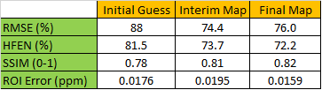
Table 1: From left to right the different image quality measure values (for the maps shown in Figure 1) are listed. RMSE is the root mean squared error. HFEN is the high-frequency error norm. SSIM is the structural similarity index. The ROI error is the absolute value of the mean error in selected anatomical structures as in the 2016 Reconstruction Challenge.
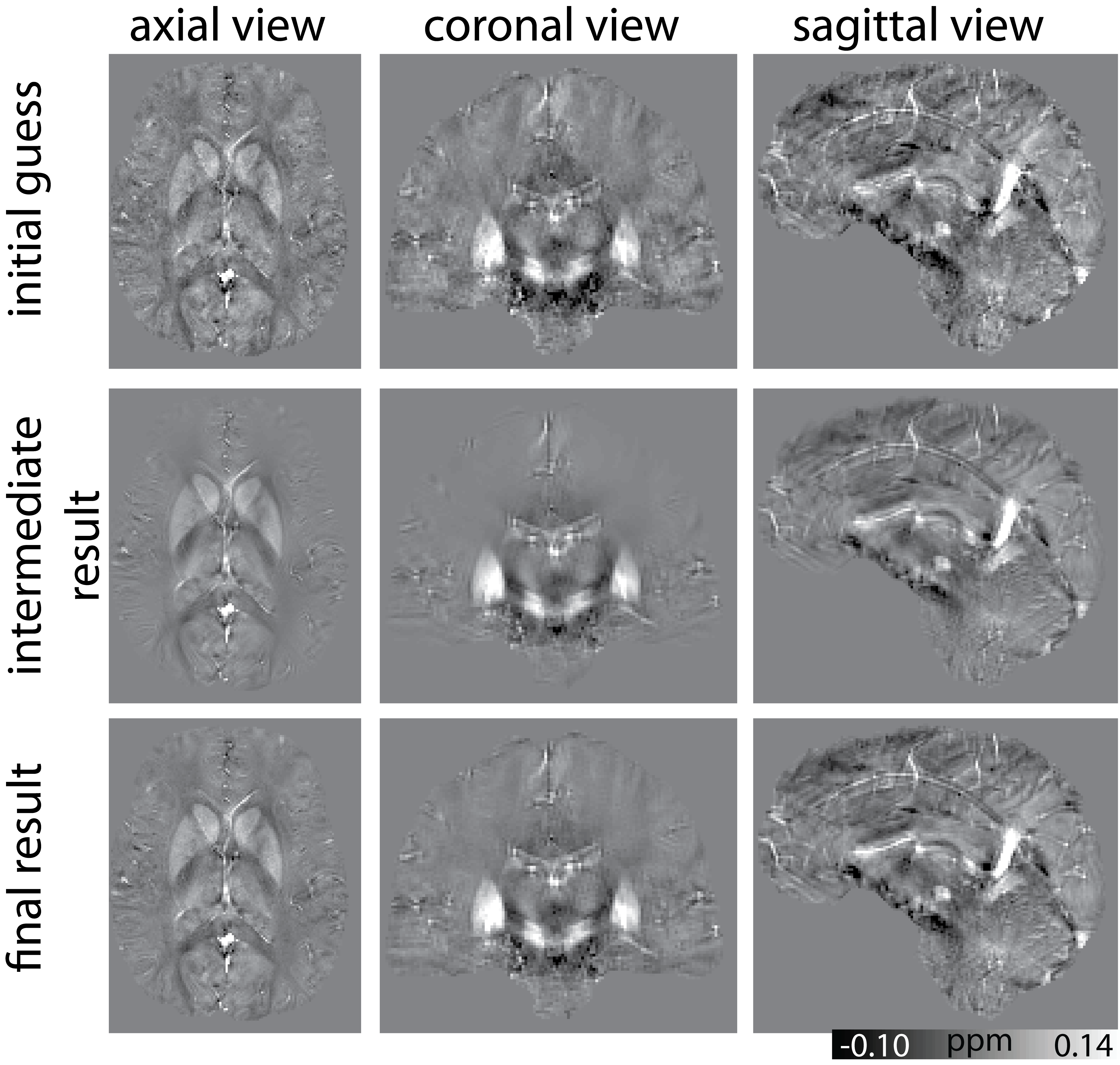
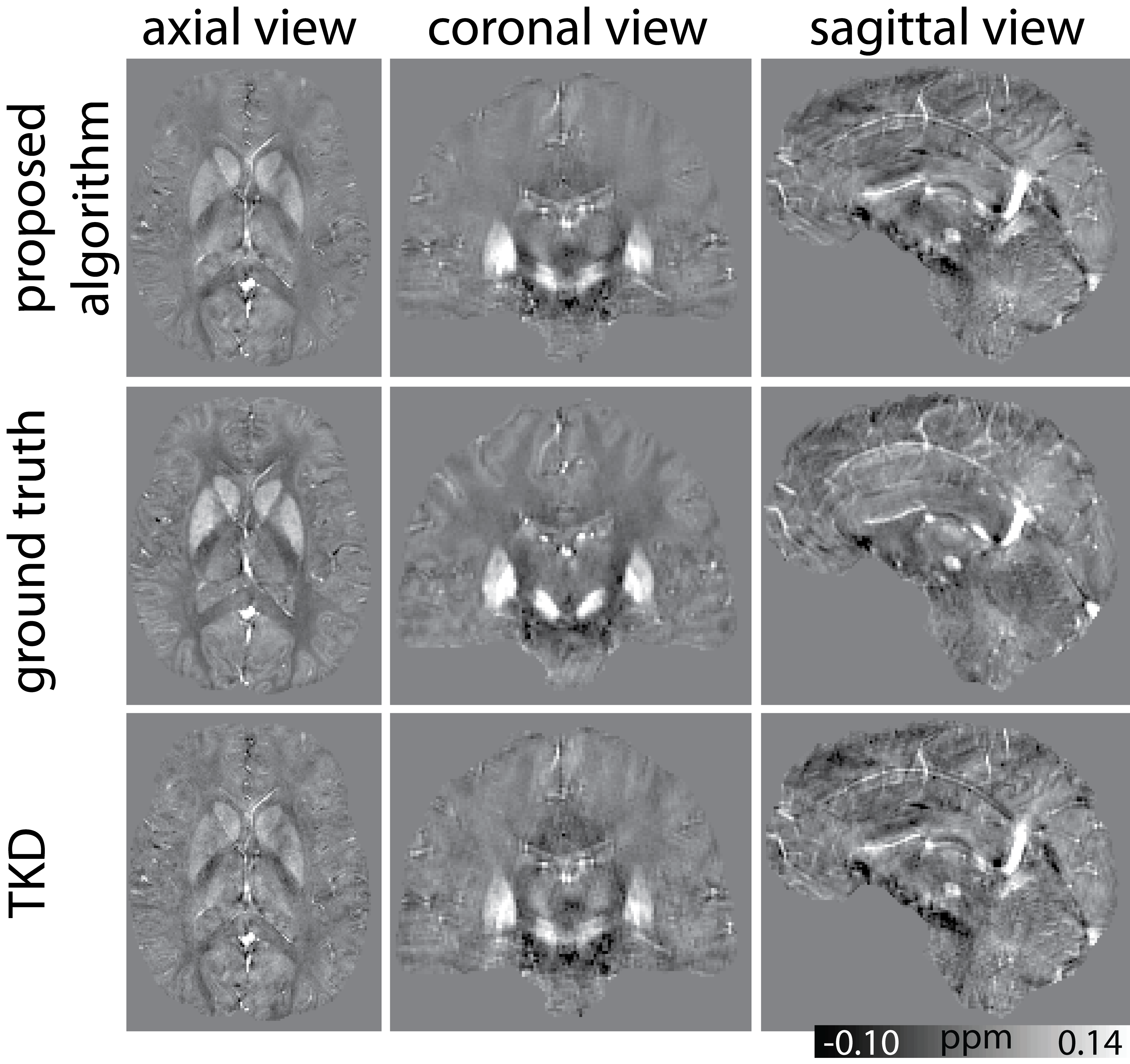
Figure 2: In the first row the axial, coronal and sagittal views of the final susceptibility maps obtained by the proposed algorithm are shown.
The second row shows the $$$\chi_{33}$$$ ground truth, and in the third row a susceptibility map calculated with truncated k-space division (TKD) is shown.