3236
Parameter estimation with matrix-based signal models using VARPRO for transient- and steady-state imaging1Biomedical Engineering, University of Southern California, Los Angeles, CA, United States, 2Electrical and Computer Engineering, University of Southern California, Los Angeles, CA, United States
Synopsis
VARPRO-based parameter estimation is extensively used in MR for its improved accuracy, precision, and convergence behavior compared to general nonlinear least-squares algorithms. This study investigates the feasibility of using matrix-based signal models with VARPRO instead of conventional analytic signal equations. Simulations and in-vivo study show that VARPRO with matrix-based signal models is identical to VARPRO with analytic signal equations, and both VARPRO approaches provide enhanced precision and accuracy in relaxometry maps compared to the conventional DESPOT1/2 methods from variable flip angle SPGR and bSSFP measurements.
Introduction
The recently introduced matrix-based signal modeling approach1 is attractive because closed-form expressions based on the Bloch equations can model off-resonance, finite duration RF pulses, and magnetization transfer effects. However, parameters were estimated by a general nonlinear least-squares algorithm with many initial starting points, which may cause convergence issues. The variable projection (VARPRO) algorithm2,3 has been proposed to provide a better convergence for "separable" least-squares problems. The VARPRO approach has been used extensively in MR4,5,6 because of its accuracy and precision for a parametric fitting of the data with analytic signal models. Here, we investigate VARPRO-based parameter estimation using matrix-based signal models for transient- and steady-state quantitative imaging.Theory
Jaynes' matrix formalism11: We assume a single-pool model. We assume that an RF pulse is applied on the x-axis with instantaneous pulse approximation. The temporal evolution of the magnetization $$$\mathbf{M}=\begin{bmatrix}M_x&M_y&M_z\end{bmatrix}^T$$$ is governed by:$$\frac{d\mathbf{M}(t)}{dt}=\left(\Omega(t)+\Lambda\right)\mathbf{M}(t)+\mathbf{C}M_0,$$where$$\Omega(t)=\begin{bmatrix}0&0&-\gamma B_{1,y}(t)\\0&0&\gamma B_{1,x}(t)\\\gamma B_{1,y}(t)&-\gamma B_{1,x}(t)&0\end{bmatrix},\Lambda=\begin{bmatrix}-R_2&2\pi\Delta f&0\\-2\pi\Delta f&-R_2&0\\0&0&-R_1\end{bmatrix},\mathbf{C}=\begin{bmatrix}0\\0\\R_1\end{bmatrix}.$$ The matrix $$$\mathbf{\Omega}(t)$$$ describes RF rotation, and $$$\mathbf{\Lambda}$$$ and $$$\mathbf{C}$$$ describe evolution in the absence of RF. A general solution to the Bloch equations in the absence of RF is described by $$$\mathbf{M}(t+\tau)=\mathbf{S}\mathbf{M}(t)+\left(\mathbf{S}-\mathbf{I}\right)\Lambda^{-1}\mathbf{C}M_0$$$ where $$$\mathbf{S}=\mathrm{exp}(\Lambda\tau)=\mathbf{E}(\tau)\mathbf{P}(\tau)$$$. The relaxation $$$\mathbf{E}(\tau)$$$ and free precession $$$\mathbf{P}(\tau)$$$ operators are defined as:$$\mathbf{E}(\tau)=\begin{bmatrix}e^{-\tau\cdot R2}&0&0\\0&e^{-\tau\cdot R2}&0\\0&0&e^{-\tau\cdot R1}\end{bmatrix},\mathbf{P}(\tau)=\begin{bmatrix}\mathrm{cos}(2\pi\Delta f\tau)&\mathrm{sin}(2\pi\Delta f\tau)&0\\-\mathrm{sin}(2\pi\Delta f\tau)&\mathrm{cos}(2\pi\Delta f\tau)&0\\0&0&1\end{bmatrix}.$$
Steady-state imaging: In the steady state, we have $$$\mathbf{R}\Psi\mathbf{M}(t+\tau)=\mathbf{M}(t)=\mathbf{M}^{SS}$$$ where $$$\mathbf{R}=\mathrm{exp}(\Omega\tau)$$$ and $$$\Psi$$$ accounts for perfect spoiling (SPGR) or $$$\pi$$$ phase cycling (bSSFP). Using the steady-state condition, we can express the steady-state magnetiztion immediately after an RF pulse as: $$$\mathbf{M}^{SS}=\left(\mathbf{I}-\mathbf{R}\Psi\mathbf{S}\right)^{-1}\mathbf{R}\Psi\left(\mathbf{S}-\mathbf{I}\right)\Lambda^{-1}\mathbf{C}M_0$$$.The matrix-based signal expressions for SPGR and bSSFP (at TE) are expressed as:$$\mathbf{M}^{SPGR}=\left(\mathbf{I}-\mathbf{R}\Psi^{SPGR}\mathbf{E}_1\mathbf{P}_1\right)^{-1}\mathbf{R}\Psi^{SPGR}\left(\mathbf{E}_1\mathbf{P}_1-\mathbf{I}\right)\Lambda^{-1}\mathbf{C}M_0$$ $$\mathbf{M}^{bSSFP}=\left(\mathbf{E}_2\mathbf{P}_2\left(\mathbf{I}-\mathbf{R}\Psi^{bSSFP}\mathbf{E}_1\mathbf{P}_1\right)^{-1}\mathbf{R}\Psi^{bSSFP}\left(\mathbf{E}_1\mathbf{P}_1-\mathbf{I}\right)\Lambda^{-1}\mathbf{C}+\left(\mathbf{E}_2\mathbf{P}_2-\mathbf{I}\right)\Lambda^{-1}\mathbf{C}\right)M_0,$$where $$$\mathbf{P}_1=\mathbf{P}(\mathrm{TR}),\mathbf{P}_2=\mathbf{P}(\mathrm{TE}),\mathbf{E}_1=\mathbf{E}(\mathrm{TR}),\mathbf{E}_2=\mathbf{E}(\mathrm{TE})$$$, $$$\Psi^{SPGR}$$$=diag([0 0 1]), and $$$\Psi^{bSSFP}$$$=diag([-1 -1 1]).
VARPRO formulation: The VARPRO method efficiently solves nonlinear least-squares problems when a general nonlinear model can be formulated as$$\min_{\alpha\in S_{\alpha},c\in S_{c}}\left\|y-\Phi(\alpha)c\right\|_2^2,$$ where $$$\mathbf{\Phi}(\alpha)$$$ is the real-valued system matrix parameterized by nonlinear parameters $$$\alpha$$$ and $$$c$$$ real-valued vector of linear parameters. For given $$$\alpha$$$, we estimate $$$c=\Phi^{\dagger}(\alpha)y$$$ and replace $$$c$$$ in the original formulation as:$$\min_{\alpha\in S_{\alpha}}\left\|y-\Phi(\alpha)c\right\|_2^2=\left\|y-\Phi(\alpha)\Phi^{\dagger}(\alpha)y\right\|_2^2=\left\|\left(\mathrm{I}-\Phi(\alpha)\Phi^{\dagger}(\alpha)\right)y\right\|_2^2.$$The subproblem with nonlinear parameters is solved with a nonlinear least-squares algorithm (e.g., Levenberg-Marquardt) with the Frechet derivative of the $$$(\mathrm{I}-\Phi(\alpha)\Phi^{\dagger}(\alpha))y$$$. The differentiation of pseudo-inverses $$$\Phi^\dagger(\alpha)$$$ with respect to $$$\alpha$$$ is well described by Golub and Pereyra2. The VARPRO formulation updates ($$$c^{(i)},\alpha^{(i)}$$$) until a stopping criteria is met. The MATLAB implementation of VARPRO8 (varpro.m) requires two inputs: $$$\Phi(\alpha)$$$ and $$$\frac{\partial\mathbf{\Phi}}{\partial\alpha}$$$. We describe the system matrices for the variable-flip-angle (VFA) SPGR, bSSFP, SPGR & bSSFP, and SPGR & bSSFP with off-resonance as:
$$\Phi(\alpha_1)^{SPGR}=\begin{bmatrix}\Omega_y\left(M^{SPGR}(\theta_1)\right)/M_0\\\Omega_y\left(M^{SPGR}(\theta_{m_1}\right)/M_0\end{bmatrix},\Phi(\alpha_2)^{bSSFP}=\begin{bmatrix}\Omega_y\left(M^{bSSFP}(\theta_1)\right)/M_0\\\Omega_y\left(M^{bSSFP}(\theta_{m_2})\right)/M_0\end{bmatrix},\\\Phi(\alpha_3)^{S\&b}=\begin{bmatrix}\Omega_y\left(M^{SPGR}(\theta_1)\right)/M_0\\\Omega_y\left(M^{SPGR}(\theta_{m_1})\right)/M_0\\\Omega_y\left(M^{bSSFP}(\theta_1)\right)/M_0\\\Omega_y\left(M^{bSSFP}(\theta_{m_2})\right)/M_0\end{bmatrix},\Psi(\alpha_4)^{S\&b,\Delta f}=\begin{bmatrix}\Omega_y\left(M^{SPGR}(\theta_1)\right)/M_0\\\Omega_y\left(M^{SPGR}(\theta_{m_1})\right)/M_0\\\Omega_x\left(M^{bSSFP}(\theta_1)\right)/M_0\\\Omega_x\left(M^{bSSFP}(\theta_{m_2})\right)/M_0\\\Omega_y\left(M^{bSSFP}(\theta_1)\right)/M_0\\\Omega_y\left(M^{bSSFP}(\theta_{m_2})\right)/M_0\end{bmatrix},$$where nonlinear parameters for each case are $$$\alpha_{1}=R_1,\alpha_{2}=R_2,\alpha_{3}=[R_1\,R_2]$$$, and $$$\alpha_{4}=[R_1\,R_2\,\Delta f]$$$, $$$\Omega_x(\cdot)$$$ and $$$\Omega_y(\cdot)$$$ select the x and y components of the magnetization, respectively, and $$$m_1$$$ and $$$m_2$$$ is the number of variable flip angles for SPGR and bSSFP, respectively. Note that $$$c=M_0$$$ for all cases and when model parameters were not included in $$$\alpha$$$, fixed parameters were assumed ($$$R_1=R_{1,true}$$$ and $$$\Delta f=0$$$ for $$$\Psi^{bSSFP}(\alpha)$$$). The derivatives of $$$\mathbf{\Phi}(\alpha)$$$ with respect to each element of $$$\alpha$$$ is defined as:$$\frac{\partial\mathbf{\Phi}}{\partial\alpha}=\left[\frac{\partial\mathbf{\Phi}}{\partial\alpha_1}\frac{\partial\mathbf{\Phi}}{\partial\alpha_2}\frac{\partial\mathbf{\Phi}}{\partial\alpha_p}\right]\in\mathbb{R}^{m\times p}.$$Each column can be calculated using the product rule and the fact that $$$\frac{d}{d\alpha}[A(\alpha)^{-1}]=-A(\alpha)^{-1}\left[\frac{d}{d\alpha}A(\alpha)\right]A(\alpha)^{-1}$$$ and $$$\left[\frac{d}{d\alpha}A(\alpha)\right]_{ij}=\frac{d}{d\alpha}A_{ij}(\alpha)$$$.
Methods
For both simulations and in-vivo experiments, excitation flip angles for SPGR were: 1.5°, 2.2°, 3.23°, 4.74°, 6.96°, 10.22°, 15° and for bSSFP were: 15° to 65° (steps of 10°).Noiseless 1D signal simulation: To test the convergence (accuracy) of the proposed method, we evaluated the proposed method on noiseless simulated datasets. Four test datasets were generated: 1) VFA SPGR, 2) VFA bSSFP, 3) VFA SPGR & bSSFP, and 4) VFA SPGR & bSSFP with off-resonance (30Hz). The datasets 1-3 and dataset 4 were generated with the Ernst and Freman-Hill equations, and a matrix-based signal model, respectively.
Noisy Brainweb simulation: We performed noisy simulation studies using a Brainweb "fuzzy" (partial volume) dataset (T1,T2,M0): We generated 1) VFA SPGR, 2) VFA SPGR & bSSFP.
Human VFA SPGR: A 3D whole-brain VFA SPGR dataset with TR = 5ms was acquired at 3T. Bloch-Siegert-based B1 maps were acquired for B1+ compensation9.
Parameter estimation: Datasets were fitted with VARPRO with matrix-based signal models (eigenvalue), VARPRO with analytic signal equations (analytic), and the conventional DESPOT1/2 method10. For both VARPRO approaches, the same initial starting points (1,1) and stopping criteria were used throughout different voxels.
Results and Discussion
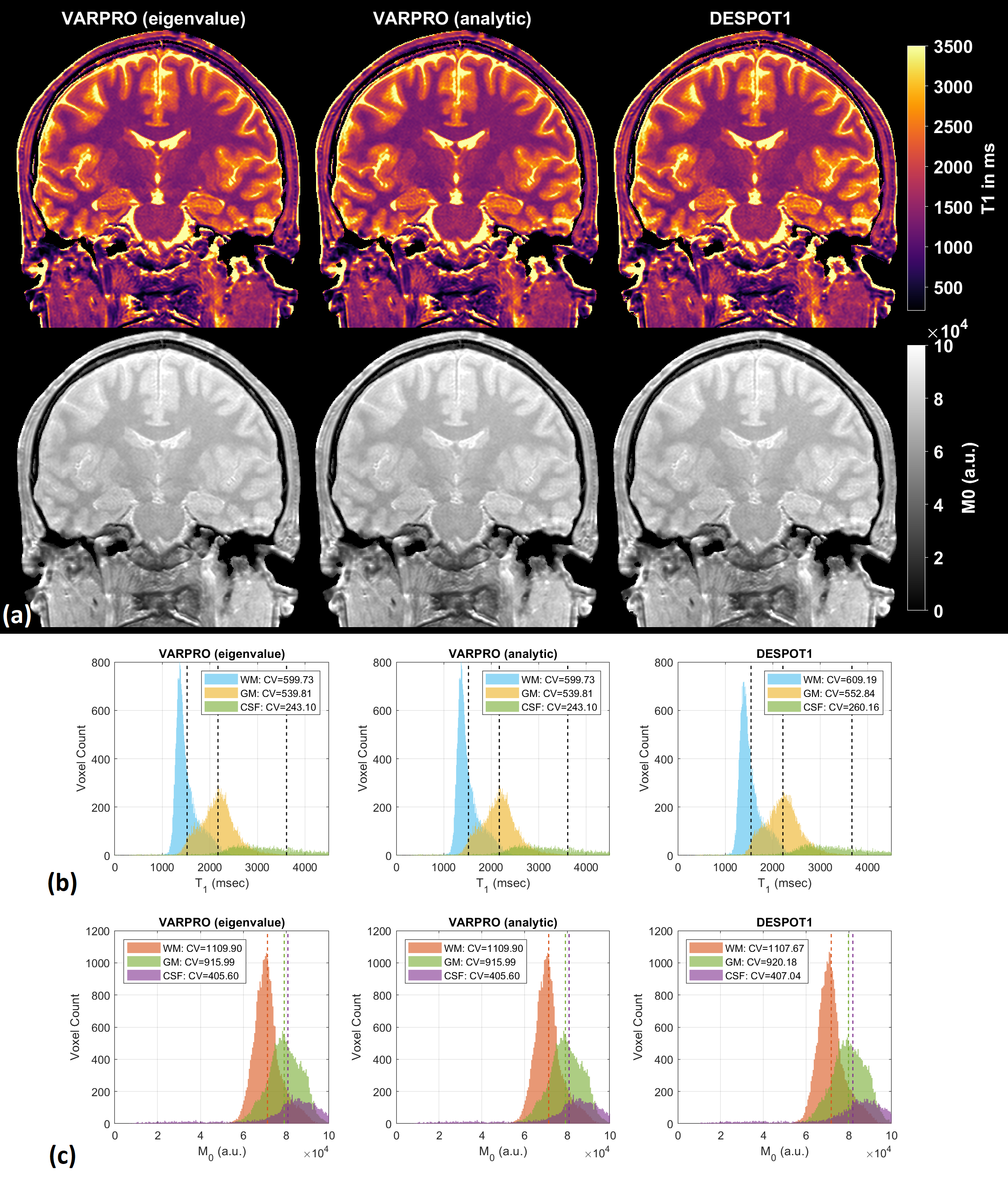
Figure 1 shows results from noiseless simulated datasets; The eigenvalue approach converged to the ground truth within a few iterations (<6) for all test cases (See legend for estimated parameters). All methods fit the data well with near-zero residual, however, only the eigenvalue VARPRO approach had no bias in all cases. Note also that the eigenvalue VARPRO approach can simultaneously estimate off-resonance (Figure 1d). Figures 2 and 3 show results from noisy simulated VFA SPGR and VFA SPGR & bSSFP Brainweb datasets, respectively; Both VARPRO approaches provide T1/T2/M0 estimates with superior accuracy and precision than DESPOT1/2. Figure 4 shows estimated T1/M0 maps from one healthy human VFA SPGR dataset; T1 histograms have lower coefficient of variation with the proposed approach suggesting that they may be more accurate. A comparison with a reference method is future work.Conclusion
We demonstrate and validate an eigenvalue VARPRO approach for parameter estimation, specifically T1/T2/M0 mapping. We show improved accuracy and precision compared to DESPOT1/2 and robustness to off-resonance compared to analytic VARPRO.Acknowledgements
We gratefully acknowledge funding support from NIH R01-HL130494.References
1. Malik SJ, A.G. Teixeira RP, West DJ, Wood TC, Hajnal JV. Steady-state imaging with inhomogeneous magnetization transfer contrast using multiband radiofrequency pulses. Magn. Reson. Med. 2019;00:1-15. doi:10/1002/mrm.27984
2. Golub GH, Pereyra V. The differentiation of pseudoinverses and nonlinear least squares problems whose variables separate. SIAM Journal on Numerical Analysis. 1973;10:413–432.
3. Golub GH, Pereyra V. Separable nonlinear least squares: The variable projection method and its applications. Inverse Prob. 2003;19:R1–R26.
4. Haldar JP, Anderson J, Sun SW. Maximum likelihood estimation of T1 relaxation parameters using VARRO. In Proceedings of the 15thAnnual Meeting of ISMRM, Berlin, Germany, 2007 (Abstract 41).
5. Hernando D, Haldar JP, Sutton BP, Ma J, Kellman P, Liang ZP. Joint estimation of water/fat images and field inhomogeneity map. Magn Reson Med. 2008;59:571–580.
6. Zhao B, Lu W, Hitchens TK, Lam F, Ho C, Liang ZP. Accelerated MR parameter mapping with low-rank and sparsity constraints. Magn Reson Med. 2015;74:489–498.
7. A.G. Teixeira RP, Malik SJ, Hajnal JV. Fast quantitative MRI using controlled saturation magnetization transfer. Magn. Reson. Med. 2018;1–14. doi:10.1002/mrm.27442
8. O’Leary DP, Rust BW. Variable projection for nonlinear least squares problems. Comput. Optim. Appl. 2013;54(3):579-593.
9. Sacolick LI, Wiesinger F, Hancu I, Vogel MW. B1 mapping byBloch–Siegert shift. Magn Reson Med 2010;63:1315–1322.
10. Deoni S, Rutt BK, Peters TM. Rapid combined T1 and T2 mapping using gradient recalled acquisition in the steady state. Magn Reson Med. 2003;49:515‐526.
11. Jaynes ET. Matrix treatment of nuclear induction. Phys. Rev. 1955;98:1099–1105 doi:10.1103/PhysRev.98.1099.
Figures
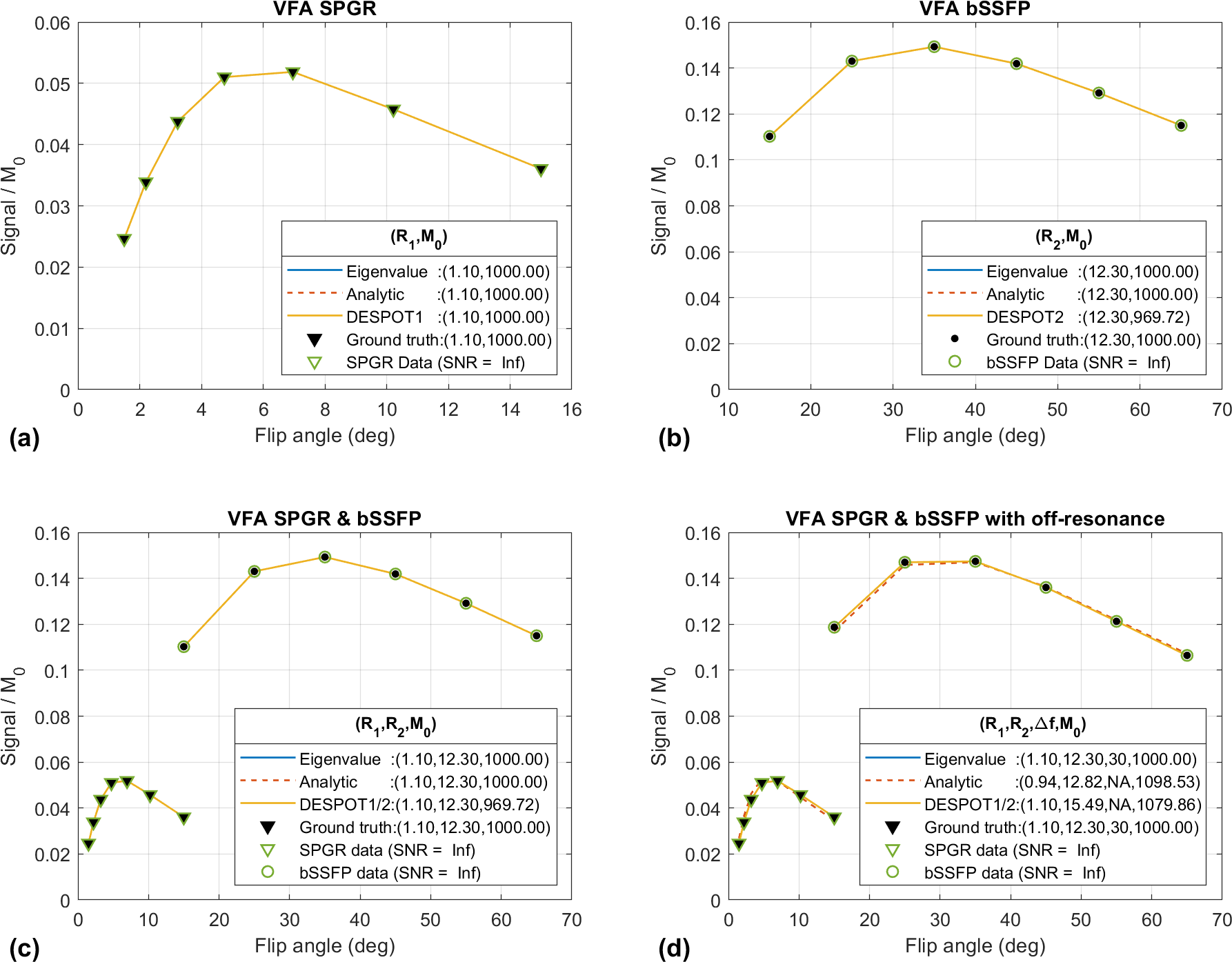
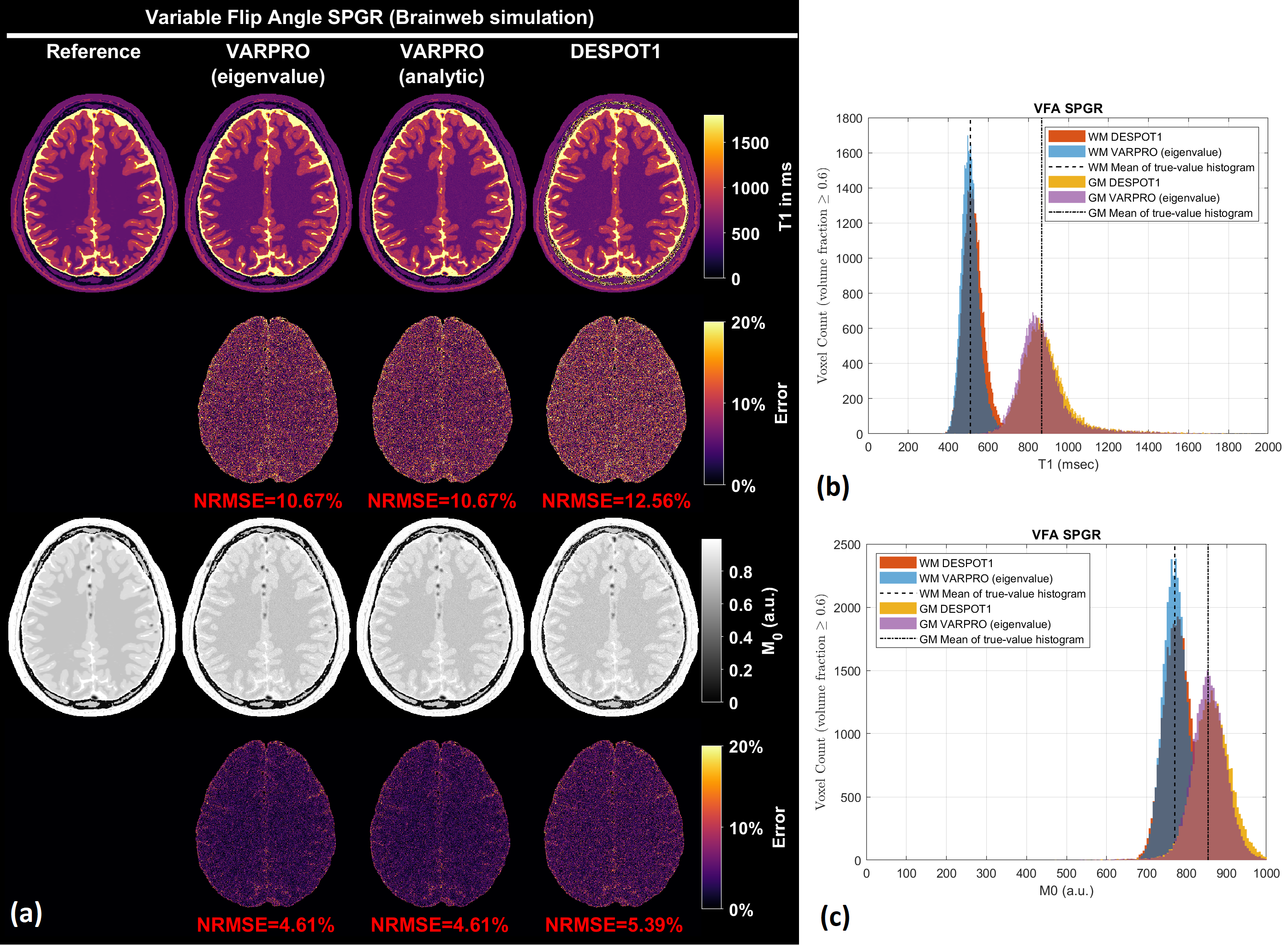
Figure 2. (a) T1 maps and M0 maps estimated by VARPRO (eigenvalue), VARPRO (analytic), and DESPOT1 from noisy simulated VFA SPGR images. Normalized voxelwise error maps are also shown. The overall normalized root-mean-square error (NRMSE) calculated within the brain is indicated in red. (b) White matter (WM) and gray matter (GM) T1 histograms. (c) WM and GM M0 histograms. The analytic approach resulted in the same parameter estimates as the eigenvalue approach and hence omitted.