INTRODUCTION

The electrical properties of biological tissues may vary depending on the anatomical structure or physiological state of tissues^1,2. Conductivity images create a unique contrast including information which is not found in other imaging modalities. DT-MREIT is an imaging modality used to image the low-frequency anisotropic conductivity distribution biological tissues^3,4,5. In this method the linear relationship between the diffusion $$$(\overline{\overline{D}})$$$ and conductivity $$$(\overline{\overline{C}})$$$ tensors in a porous medium is exploited:
$$\overline{\overline{C}}=\eta\overline{\overline{D}}\space\space\space\space\space\space\space\space\space\space(1)$$
Where $$$\eta$$$ is the extra-cellular conductivity and diffusivity ratio (ECDR). In almost all of the DT-MREIT applications in the literature two current injection patterns are used to reconstruct $$$\eta$$$. In this study, a new approach is proposed to reconstruct $$$\eta$$$ using only a single current injection.

METHODS

To reconstruct $$$\eta$$$ distribution, electrical current is injected to the imaging medium. The resultant current density distribution $$$\overline{J}$$$ for each pixel is given by:
$${\overline{J_{i}}}=-\overline{\overline{C}}{\nabla\phi_i}=-\eta\overline{\overline{D}}{\nabla\phi_i}\space\space\space\space\space\space\space\space\space\space(2)$$
where $$$i$$$ represents the $$$i^{th}$$$ current injection profile and $$$\phi_i$$$ is the scalar electrical potential corresponding to $$$\overline{J}_{i}$$$. The curl-free condition of the electric field at low frequencies³ results in:
$$\tilde{\nabla}\times(\overline{\overline{D}}\space^{-1}{\overline{J}_{i}})=\tilde{\nabla}ln(\eta)\times(\overline{\overline{D}}\space^{-1}\overline{J}_i)\space\space\space\space\space\space\space\space\space\space(3)$$
where $$$\tilde{\nabla}=(\frac{\partial}{\partial{x}},\frac{\partial}{\partial{y}})$$$. For two linearly independent current injection profiles, Eq.3 can be expressed for each pixel as:
$$\begin{bmatrix}(\overline{\overline{D}}\space^{-1}{\overline{J}_{1}})_y&-(\overline{\overline{D}}\space^{-1}{\overline{J}_{1}})_x\\(\overline{\overline{D}}\space^{-1}{\overline{J}_{2}})_y&-(\overline{\overline{D}}\space^{-1}{\overline{J}_{2}})_x\end{bmatrix}_{2\times2}\begin{bmatrix}\frac{\partial{ln(\eta)}}{\partial{x}}\\\frac{\partial{ln(\eta)}}{\partial{y}}\end{bmatrix}_{2\times1}=\begin{bmatrix}\frac{\partial(\overline{\overline{D}}\space^{-1}{\overline{J}_{1}})_x}{\partial{y}}-\frac{\partial(\overline{\overline{D}}\space^{-1}{\overline{J}_{1}})_y}{\partial{x}}\\\frac{\partial(\overline{\overline{D}}\space^{-1}{\overline{J}_{2}})_x}{\partial{y}}-\frac{\partial(\overline{\overline{D}}\space^{-1}{\overline{J}_{2}})_y}{\partial{x}}\end{bmatrix}_{2\times1}\space\space\space\space\space\space\space\space\space\space(4)$$
By solving Eq.4, $$$\tilde{\nabla}ln(\eta)$$$ is obtained. To recover $$$\eta$$$ from $$$\tilde{\nabla}ln(\eta)$$$, two iterative methods have been proposed in, ^3,5.
To reconstruct $$$\eta$$$ using a single current injection, first-order discrete approximations of $$$x$$$ and $$$y$$$ gradient operators i.e., $$$\overline{\overline{\delta}}_x$$$ and $$$\overline{\overline{\delta}}_y$$$^6,7 are utilized. For single current injection Eq.4 can be expressed as:
$$\begin{bmatrix}(\overline{\overline{D}}\space^{-1}{\overline{J}_{1}})_y&-(\overline{\overline{D}}\space^{-1}{\overline{J}_{1}})_x\end{bmatrix}_{1\times2}\begin{bmatrix}\frac{\partial{ln(\eta)}}{\partial{x}}\\\frac{\partial{ln(\eta)}}{\partial{y}}\end{bmatrix}_{2\times1}=\begin{bmatrix}\frac{\partial(\overline{\overline{D}}\space^{-1}{\overline{J}_{1}})_x}{\partial{y}}&-\frac{\partial(\overline{\overline{D}}\space^{-1}{\overline{J}_{1}})_y}{\partial{x}}\end{bmatrix}_{1\times1}\space\space\space\space\space\space\space\space\space\space(5)$$
By expanding Eq.5 for the entire imaged slice with $$$N$$$ pixels we have:
$$\overline{\overline{A}}_{N\times{N}}ln(\overline{\eta})_{N\times1}=\overline{c}_{N\times1}\space\space\space\space\space\space\space\space\space\space(6)$$
where
$$\overline{\overline{A}}=diag(\overline{a}_1)\overline{\overline{\delta}}_x+diag(\overline{a}_2)\overline{\overline{\delta}}_y,\\\overline{a}_1=\begin{bmatrix}(\overline{\overline{D}}\space^{-1}{\overline{J}_{1}})_{y,1}\\\vdots\\(\overline{\overline{D}}\space^{-1}{\overline{J}_{1}})_{y,N}{}\end{bmatrix}_{N\times1},\space\space\space\space\space\overline{a}_2=\begin{bmatrix}(\overline{\overline{D}}\space^{-1}{\overline{J}_{1}})_{x,1}\\\vdots\\(\overline{\overline{D}}\space^{-1}{\overline{J}_{1}})_{x,N}{}\end{bmatrix}_{N\times1},\\\overline{c}=\begin{bmatrix}{(\frac{\partial(\overline{\overline{D}}\space^{-1}{\overline{J}_{1}})_x}{\partial{y}}-\frac{\partial(\overline{\overline{D}}\space^{-1}{\overline{J}_{1}})_y}{\partial{x}})_1}\\\vdots\\{(\frac{\partial(\overline{\overline{D}}\space^{-1}{\overline{J}_{1}})_x}{\partial{y}}-\frac{\partial(\overline{\overline{D}}\space^{-1}{\overline{J}_{1}})_y}{\partial{x}})_N}{}\end{bmatrix}_{N\times1}\space\space\space\space\space\space\space\space\space\space(7)$$
and $$$diag(\overline{v})$$$ returns a square diagonal matrix with $$$\overline{v}$$$ as the main diagonal. In Eq.6, $$$\overline{\eta}$$$ is the vector composed of scalar $$$\eta$$$ values of all pixels in the imaged slice. Each entry of $$$\overline{a}_1$$$, $$$\overline{a}_2$$$ and $$$\overline{c}$$$ are obtained from a single pixel in the imaged slice. To solve Eq.7, Tikhonov regularized least squares solution is used with L-curve to choose regularization parameter⁸.

RESULTS

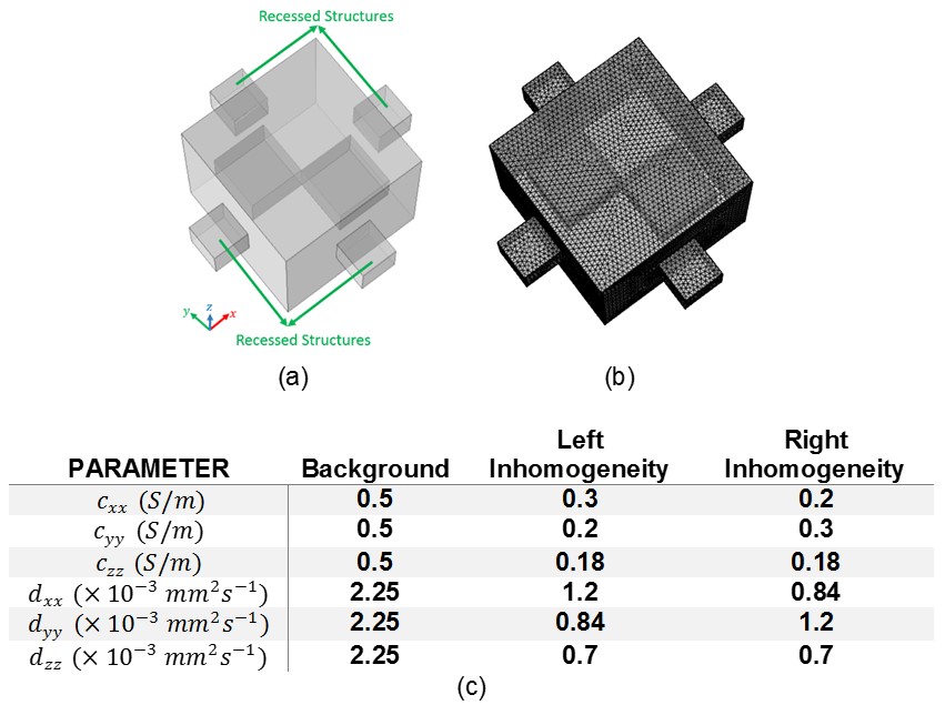
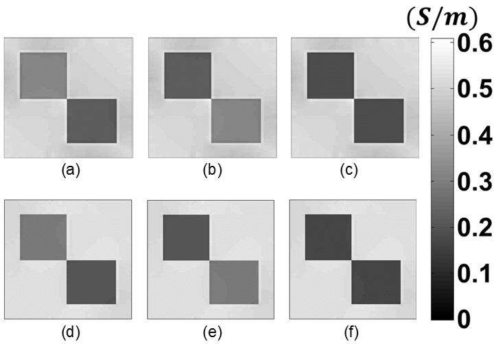
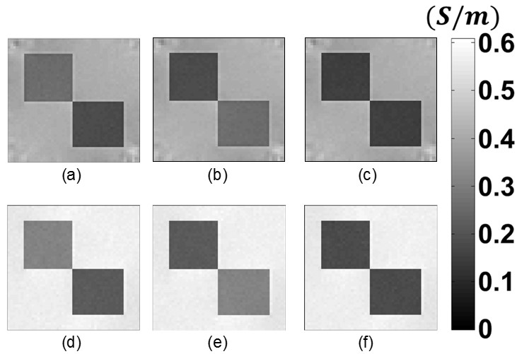
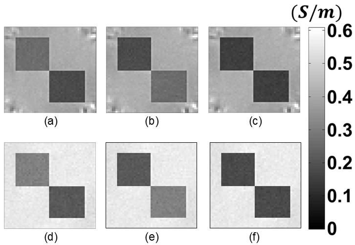
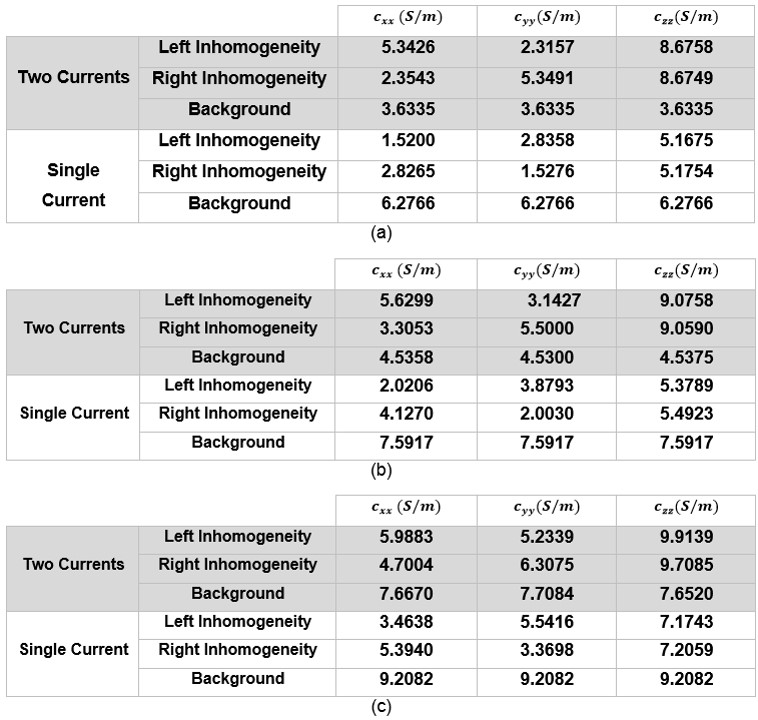
The performance of the proposed method is evaluated using simulated data for different SNR levels and the results are compared to method with two current injections in, ³. A FE model is constructed using COMSOL Multiphysics 5.1 (COMSOL AB, Sweden) as shown in Fig.1(a-b). Anisotropic conductivity and diffusion values of the FE model are given in Fig.1(c).
The diagonal components of the reconstructed conductivity tensor using two current injections (method in, ³ implemented in, ⁹) and a single current injection (the proposed method) for $$$SNR=\infty$$$, $$$SNR=40dB$$$ and $$$SNR=34dB$$$ are given in Fig.2-4, respectively. To produce noisy data, White Gaussian Noise is added to the diffusion and current density data. The RMSE values (%) of the reconstructed diagonal conductivity distributions for different regions of the FE model and for different levels are given in Table 1. The RMSE values (%) are calculated as:
$$RMSE(\%)=\sqrt{\frac{1}{N}\sum_{j=1}^N\frac{(c_t^j-c_r^j)^2}{(c_t^j)^2}}\times100\space\space\space\space\space\space\space\space\space\space(8)$$
where $$$c_t^j$$$ and $$$c_r^j$$$ are the true and reconstructed conductivity values of the $$$j^{th}$$$ pixel, respectively. $$$N$$$ is the total number of pixels for each inhomogeneity object and the background of the FE model in Fig.1.

DISCUSSION

Considering the reconstructed images in Fig.2-4 and the RMSE values in Table 1, it is seen that the proposed method using a single current injection provides similar performance with the method using dual current injections in, ³. This similarity is expected since the two unknowns in Eq.4 are just the partial derivatives of ECDR in the $$$x$$$ and $$$y$$$ directions. Therefore, by approximating $$$x$$$ and $$$y$$$ gradient operators with $$$\overline{\overline{\delta}}_x$$$ and $$$\overline{\overline{\delta}}_y$$$ the problem in Eq.4 reduces to a problem with a single unknown in Eq.5. The proposed method is quite successful in dealing with noisy data reconstruction. As it is seen in Fig.3-4, the corner regions of the reconstructed conductivity images using the dual current injection method in, ³ are erroneous. These artifacts occur at corner regions where the current density becomes comparable with the noise level. This shows the increased vulnerability of the two current method in, ³ to the added noise in comparison with the proposed method with a single current injection. Although the proposed method provides better contrast images, the reconstructed background conductivity (with isotropic distribution) is slightly higher than true values with a scale factor. Considering Table 1, the proposed method shows superior performance in regions with anisotropic conductivity distribution even though only one current is injected. Besides reducing the total scan time to half, the proposed method provides a great advantage when more than one current injection is not possible due to various reasons such as patient condition.

CONCLUSION

In this study, a new approach is proposed for DT-MREIT to reconstruct the conductivity tensor images using only a single current injection. The RMSE values of the reconstructed anisotropic conductivities for $$$SNR=\infty$$$ are around 3%. Hence, the proposed method has superior performance though only one current injection is used. Moreover, the RMSE values of the reconstructed anisotropic conductivities for experimental SNR levels ($$$SNR=34dB$$$) are around 5% which shows high insensitivity of the proposed method to the additive noise. Therefore, the clinical practicality of DT-MREIT can be enhanced by the reduction of current injection patterns without any deterioration of the obtained results.

References

1. Surowiec AJ, Stuchly SS, Barr JR, Swarup AA. Dielectric properties of breast carcinoma and the surrounding tissues. IEEE Transactions on Biomedical Engineering. 1988 Apr;35(4):257-263.
2. Joines WT, Zhang Y, Li C, Jirtle RL. The measured electrical properties of normal and malignant human tissues from 50 to 900 MHz. Medical physics. 1994 Apr;21(4):547-550.
3. Kwon OI, Jeong WC, Sajib SZ, Kim HJ, Woo EJ. Anisotropic conductivity tensor imaging in MREIT using directional diffusion rate of water molecules. Physics in Medicine & Biology. 2014 May 19;59(12):2955-2974.
4. Chauhan M, Indahlastari A, Kasinadhuni AK, Schär M, Mareci TH, Sadleir RJ. Low-Frequency Conductivity Tensor Imaging of the Human HeadIn VivoUsing DT-MREIT: First Study. IEEE transactions on medical imaging. 2017 Dec 14;37(4):966-976.
5. Jeong WC, Sajib SZ, Katoch N, Kim HJ, Kwon OI, Woo EJ. Anisotropic conductivity tensor imaging of in vivo canine brain using DT-MREIT. IEEE transactions on medical imaging. 2016 Aug 8;36(1):124-131.
6. Sharif B, Kamalabadi F. Optimal sensor array configuration in remote image formation. IEEE Transactions on Image Processing. 2008 Jan 14;17(2):155-166.
7. Hansen PC. Discrete inverse problems: insight and algorithms. Siam; 2010 Mar 18.
8. Hansen PC. The L-curve and its use in the numerical treatment of inverse problems. Computational Inverse Problems in Electrocardiology. Advances in Computational Bioengineering. 2001;5:119.
9. Sajib SZ, Katoch N, Kim HJ, Kwon OI, Woo EJ. Software Toolbox for Low-Frequency Conductivity and Current Density Imaging Using MRI. IEEE Transactions on Biomedical Engineering. 2017 Jul 27;64(11):2505-2514.