3228
Multi-parametric quantification of multiple spectral components by an extended MR-STAT framework1Computational Imaging group for MR Diagnostics and Therapy, Center for Image Sciences, University Medical Center Utrecht, Utrecht, Netherlands
Synopsis
We present a novel method called Bicompartemental MR-STAT for simultaneous quantification T1, T2 and Proton density for two resonances based upon the MR-STAT framework. T1 and T2 may vary per compound in this framework. Additionally B0 is reconstructed by taking advantage of multple readouts within each TR which allows for separate but accurate B0 reconstruction.
Introduction
Multi-parametric methods such as MRF1 and MR-STAT 2 rely on model-based parametric reconstructions. Usually, the employed MR signal models refer to a single resonance frequency (water) inside a voxel. Although this assumption is realistic for neuro acquisitions, body MR needs to take into account also signal from fat. In this work, a bi-compartmental MR-STAT framework is presented which allows for separation of the water and fat signal contributions with the aim of eliminating the quantification biases which may results from simplistic mono-compartment models.Bi-compartemental MR-STAT is thus an extension to the MR-STAT framework where the parameters T1,T2 and Proton density for the water signal (4.7 ppm), and the dominant fat signal ( (CH2)n , 1.3 ppm) are jointly reconstructed. Additionally B0 is reconstructed by taking advantage of multiple readouts within each TR which allows for separate but accurate B0 reconstruction.
Theory
The extended MR-STAT signal model at sampling time $$$t$$$ may be written as:$$ d(t) = \int_{V} \sum_{i = 1}^N \rho^{i}(\vec{r}) M(T^{i}_1(\vec{r}), T_2^{i}(\vec{r}), B_0(\vec{r}), \omega^i,t) d^3\vec{r} $$
Where $$$ N$$$ is the number of modeled resonances and is set to 2 in this case, respectively water and methyline ((CH2, the dominant fat component) or acetone for the experimental phantom. $$$M$$$ gives the response of Bloch equation. Acquisitions follow a multi-echo strategy where two echoes are in-phase in order to maximize decorrelation of the signal. This enhances the separation of the water and fat tissues, which allows reconstruction of $$$ T^{w}_1(\vec{r}), T^{f}_1(\vec{r}), T_2^{w}(\vec{r}), T_2^{f}(\vec{r}), \rho^{w}, \rho^{f}$$$ in a cyclic fashion. Each sub-problem is solved as a separate MR-STAT problem with five iterations, see also Figure 1. By solving the inverse problem in this iterative scheme it is assumed that the calculated signals from Figure 1 converge towards true values.
$$$ B_0 $$$ is initialized in a separate preprocessing step. Since MR-STAT data is typically acquired with fully sampled Cartesian k-space and slowly-varying flip-angles, a Fourier Transform step can return images for each k-space and each echo. In this work, we implemented three readouts in each TR, two there of are timed to eliminate the phase accrual of off-resonance (fat). B0 can thus be obtained by phase data of these two echoes. Using element wise division of the Fourier Transformed in phase images, we may construct and solve the following regularized equation for $$$ B_0 $$$: $$ \arg \min_{\Delta B_0} || A(\Delta\text{TE})\vec{B_0}(r) - \vec{\phi}(r) ||^2 + ||\lambda \nabla^2 (\vec{B_0})||$$ The regularization parameter is chosen to enforce smoothness of the map.
Methods
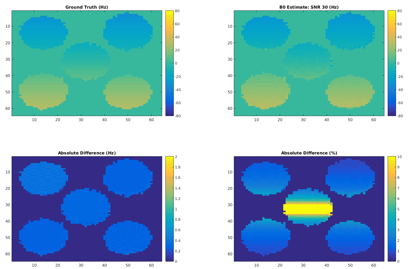
A spoiled gradient multi echo sequence with a slowly variable flip angle is proposed in this work. The echo times chosen in this work are such that the echo train is in phase, out of phase and in phase again. This implies $$$2.3 \ ms, \ 5.8\ ms$$$ and $$$ 9.3\ ms $$$ for fat and $$$3.1\ ms, \ 7.9\ ms$$$ and $$$ 12.6\ ms $$$ for Acetone at 3.0T and the echoes are acquired with alternating polarity. The TRs have been set to $$$ 11.6\ ms $$$ and $$$ 15.7\ ms $$$ respectively. The flip angle train follows a squared sine function and is shown in Figure 2 .The quantitative parameters are then solved as an inverse problem from the data using Eq. (1) and the cyclic scheme described above. An estimated $$$B_0$$$ map from the data is given as an as an input parameter for solving the bi-compartemental MR-STAT model and obtaining $$$T_{1w}, T_{1f}, T_{2w}, T_{2f}$$$ as written in the theory section. Figure 3 shows reconstructed $$$ B_0 $$$ on a digital phantom, with generated white noise such that SNR = 30.0 as well as extra resonances comparable to the extra fat resonances were added.
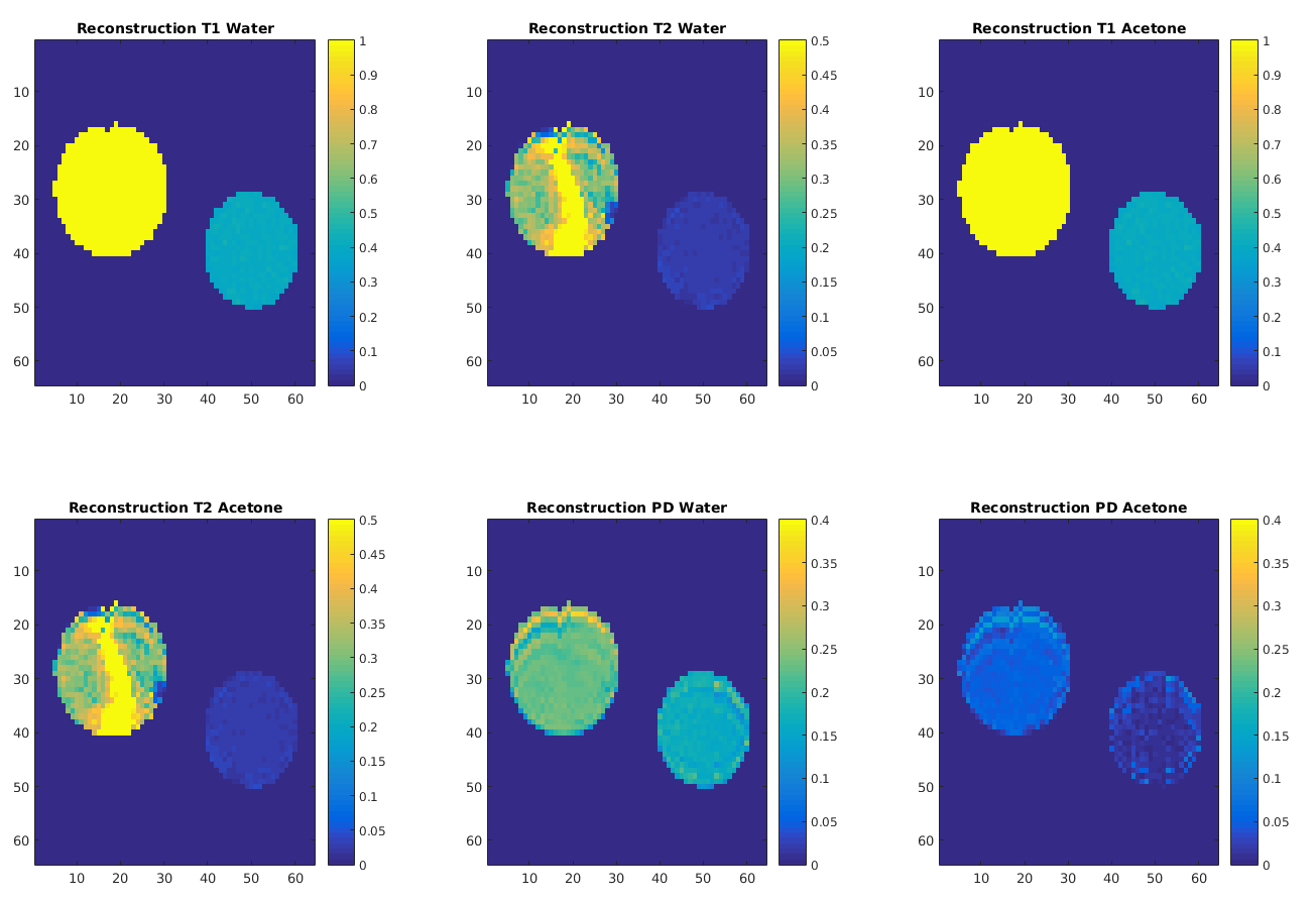
Preliminary results are also available on real data measured on an in-house made phantom next to a commercially available phantom containing only a water resonance. The in house made phantom consists of acetone mixed with water such that the proton density ratio is approximately 1:3.5. Data was acquired on a Philips Ingenia 3.0T system. Although this reconstruction failed to quantify the relaxation times properly unfortunately, it does show the merit of this method. Acetone is reconstructed only in significant amounts in the tube where it's located, and the proton density ratio recovered is between about 1:4.5. Furthermore the second phantom is reconstructed nearly uniform, which it should be. More investigation is required why this dataset has these quantification anomalies .
Conclusion and Discussion
The simulation data show that the Bi-compartemental MR-STAT method for reconstructed multiple resonances looks promising, allowing the possibility of accurate quantification for multiple signal compartments, while the experimental data show that there is merit to the method. It is currently unknown why the reconstruction on the experimental shows these results reported here, but these errors could arise from an error in measuring the Aceton Off-resonance for example. As far as the authors know there is no other method attempting to quantify different relaxation methods for different resonances. This model could be extended in the future using additional echoes wihtin the chosen sequence for more than two resonances in a similar cyclic scheme, which would make this method a potentially very powerful tool in quantification.Acknowledgements
We would like to thanks W. van de Kemp, J. Prompers and J. Wijnen for fruitful discussions and acquisition about the experimental phantom choice in this work.References
1.Assländer, J., Cloos, M. A., Knoll, F., Sodickson, D. K., Hennig, J.,
& Lattanzi, R. (2018). Low rank alternating direction method of
multipliers reconstruction for MR fingerprinting. Magnetic resonance in medicine, 79(1), 83-96
2.Sbrizzi, A., van der Heide, O., Cloos, M., van der Toorn, A., Hoogduin,
H., Luijten, P. R., & van den Berg, C. A. (2018). Fast quantitative
MRI as a nonlinear tomography problem. Magnetic resonance imaging, 46, 56-63.
Figures
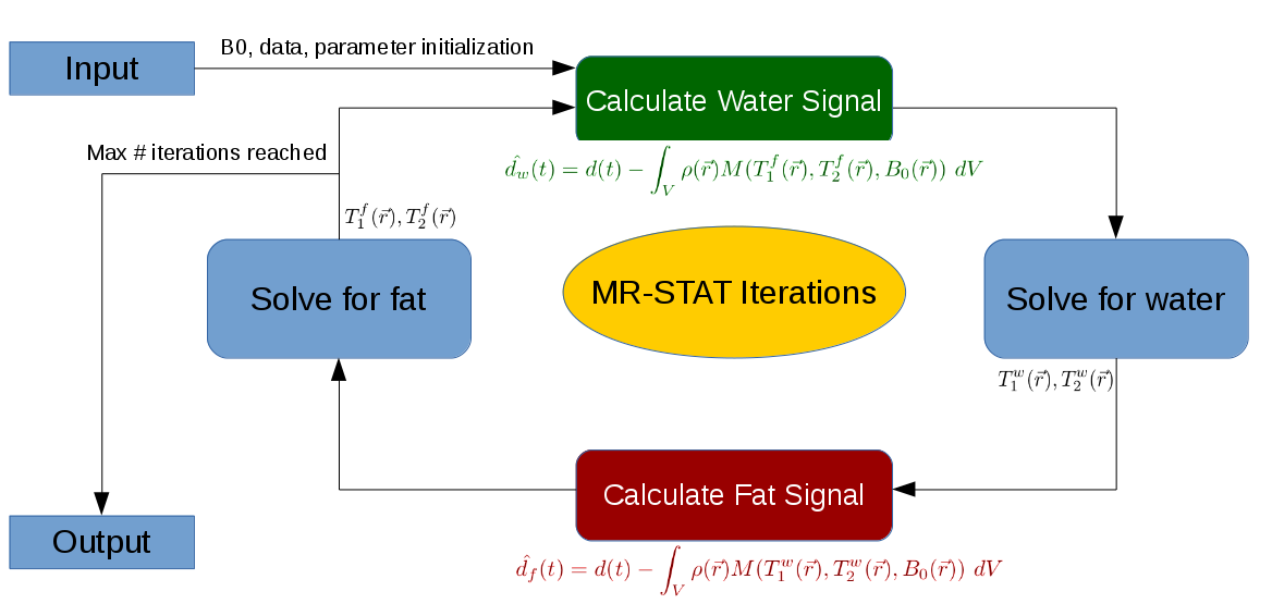
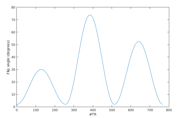
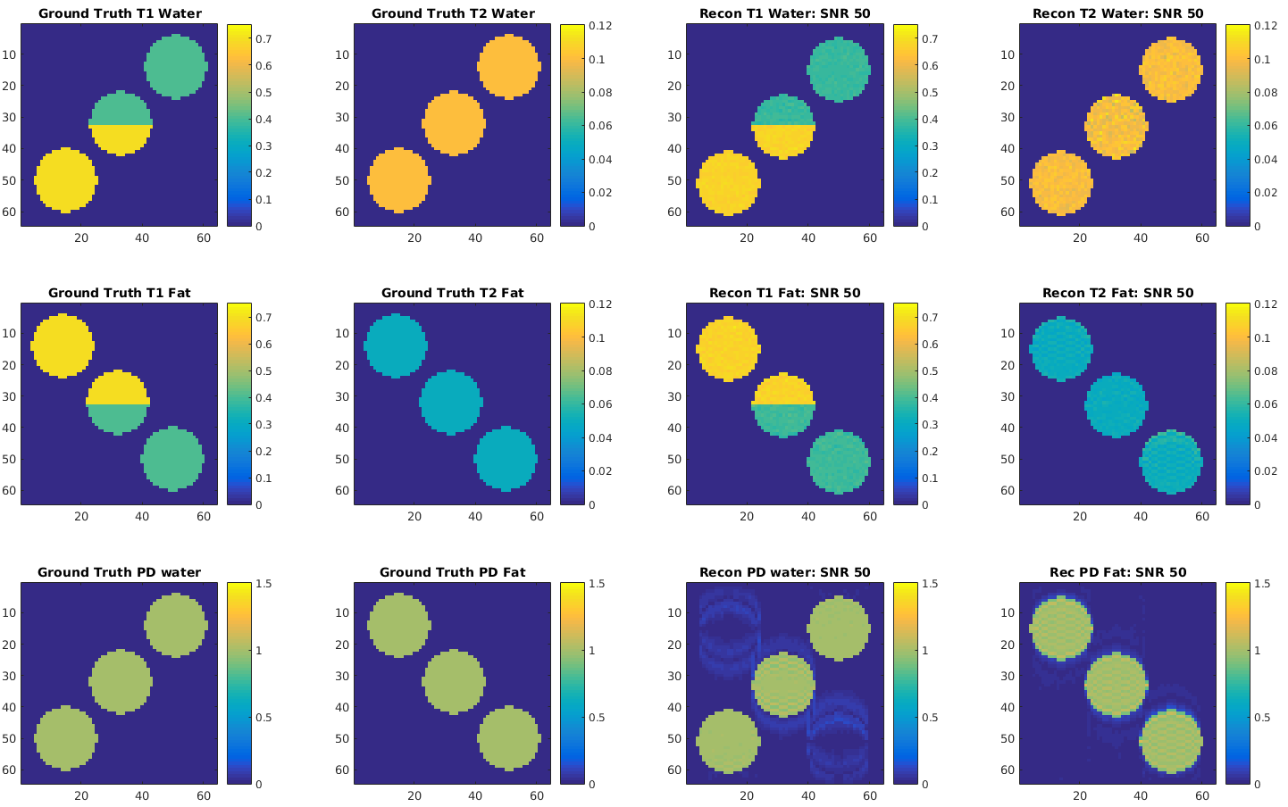
Figure 3: Reconstructions of simulated data with SNR 50 to show the concept of the method. As can be seen the reconstruction matches the ground truth very well, up to a minor bias for T1 in the order of $$$15 msec $$$.