Introduction

Conventional quantitative susceptibility mapping (QSM) algorithms have an assumption that the frequency shift is attributed only to the magnetic susceptibility effect.¹ However, several studies have demonstrated that additional sources such as chemical shift/exchange^2-4 contribute to the frequency shift and generate errors in QSM results. Recently, a simple geometric approach that separates susceptibility and chemical shift/exchange was developed using three orthogonal B₀ directional datasets.⁵ In this study, we propose two generalized methods that allow us to utilize multiple arbitrary B₀ directional dataset for the separation. Additionally, the effect of noise amplification for small B₀ angles is explored. A preliminary in-vivo result is included.

Methods

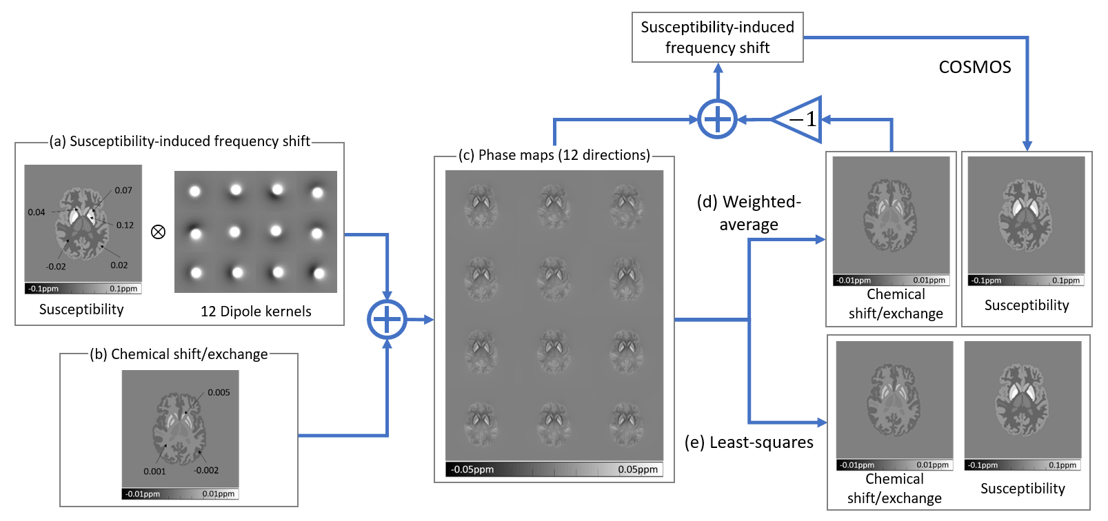
[Physics] When both susceptibility and chemical shift/exchange co-exist, the Fourier transform of resonance frequency shift with N different B₀ directions can be modeled as follows^5,6:
$$\mathit{\Delta}F_i\left(k\right)\mathrm{=}\ F_{s,i}\left(k\right)\mathrm{+}F_c\left(k\right)\mathrm{=}\ D_i\left(k\right)X\left(k\right)\mathrm{+}F_c\left(k\right),{\qquad}[Eq. 1]$$ $$D_i\left(k\right)=\frac{\mathrm{1}}{\mathrm{3}}\mathrm{-}\frac{{\left(k_z{cos{\theta}_i}\mathrm{+}k_y{sin{\theta}_i}{cos{\phi}_i}\mathrm{+}k_x{sin{\theta}_i}{sin{\phi}_i}\right)}^{\mathrm{2}}}{k^{\mathrm{2}}_x\mathrm{+}k^{\mathrm{2}}_y\mathrm{+}k^{\mathrm{2}}_z},{\qquad}[Eq. 2]$$where $$$∆F$$$ is the total frequency shift, $$$F_s$$$ is the susceptibility-induced frequency shift, $$$F_c$$$ is the chemical shift/exchange, $$$D$$$ is a dipole kernel, $$$X$$$ is susceptibility, sub-index $$$i$$$ represents a B₀ direction ($$$i$$$ = 1,2,…, and N), $$$\theta$$$ and $$$\phi$$$ are the angles of the B₀ direction in the spherical coordinate. The chemical shift/exchange is assumed not to be influenced by the B₀ direction.
[Weighted-average] The susceptibility effect can be summed to zero if we find coefficient $$${a_i}$$$ that satisfies:
$$\sum^N_i{a_iD_i(k)}=\sum^N_i{a_i\left\{\frac{1}{3}-\frac{{\left(k_z{cos{\theta}_i}+k_y{sin{\theta}_i}{cos{\phi}_i}+k_x{sin{\theta}_i}{sin{\phi}_i}\right)}^2}{k^2_x+k^2_y+k^2_z}\right\}}=0.{\qquad}[Eq. 3]$$ Equation 3 can be reformulated as follows:$$\left[\begin{array}{cccc}\frac{1}{3}-{{sin}^2{\theta}_1}{{cos}^2{\phi}_1} &{\frac{1}{3}-{{sin}^2{\theta}_2}{{cos}^2{\phi}_2}}&{\cdots}&{\frac{1}{3}-{{sin}^2{\theta}_N}{{cos}^2{\phi}_N}}\\{\frac{1}{3}-{{sin}^2{\theta}_1}{sin^2{\phi}_1}}&{\frac{1}{3}-{{sin}^2{\theta}_2}{sin^2{\phi}_2}}&{\cdots}&{\frac{1}{3}-{{sin}^2{\theta}_N}{sin^2{\phi}_N}}\\{{cos{\theta}_1}{sin{\theta}_1}{cos{\phi}_1}}&{{cos{\theta }_2}{sin {\theta}_2}{cos{\phi}_2}}&{\cdots}&{{cos{\theta}_N}{sin{\theta}_N}{cos{\phi}_N}}\\{{{sin}^2{\theta}_1}{cos{\phi}_1}{sin{\phi}_1}}&{{{sin}^2{\theta}_2}{cos{\phi}_2}{sin{\phi}_2}}&{\cdots}&{{{sin}^2{\theta}_N}{cos{\phi }_N}{sin{\phi }_N}}\\{{cos{\theta}_1}{sin{\theta}_1}{sin{\phi}_1}}&{{cos{\theta}_2}{sin{\theta}_2}{sin{\phi}_2}}&{\cdots}&{{cos{\theta}_N}{sin{\theta}_N}{sin{\phi}_N}}\end{array}\right]\left[\begin{array}{c}a_1\\a_2\\{\vdots}\\a_N \end{array}\right]=K\overrightarrow{a}=0.{\qquad}[Eq. 4]$$ When $$$K$$$ is not a full rank, the null space of $$$K$$$ includes non-zero $$$\overrightarrow{a}$$$ vectors resulting in non-trivial solutions of $$$\overrightarrow{a}$$$. Thus, the chemical shift/exchange can be measured as the weighted-average of the total frequency shift data. The susceptibility map can be reconstructed from chemical shift/exchange-removed frequency shift using COSMOS reconstruction⁷ as summarized below. $$F_c\left(k\right)=\ \frac{\sum^N_i{a_i\mathit{\Delta}F_i\left(k\right)}}{\sum^N_i{a_i}},{\qquad} F_{s,i}\left(k\right)=D_i\left(k\right)X\left(k\right)\mathrm{=}\ \mathrm{\Delta }F_i\left(k\right)-\frac{\sum^N_i{a_i\mathit{\Delta}F_i\left(k\right)}}{\sum^N_i{a_i}}.{\qquad}[Eq. 5]$$
[Least-squares] Given a set of N measurements, we can define a pointwise linear relationship between the frequency shift and the two sources. $$\left[\begin{array}{c}\mathit{\Delta}F_1\left(k\right) \\ \mathit{\Delta}F_2\left(k\right)\\{\vdots}\ \\ \mathit{\Delta}F_N\left(k\right)\end{array}\right]\mathrm{=}\left[\begin{array}{c}\begin{array}{cc}D_1\left(k\right)&1\end{array} \\ \begin{array}{cc}D_2\left(k\right)&1\end{array}\\{\vdots}\\ \begin{array}{cc}D_N\left(k\right)&1\end{array}\end{array}\right]\left[\begin{array}{c}X\left(k\right) \\F_c\left(k\right)\end{array}\right]=D\left[\begin{array}{c}X\left(k\right)\\F_c\left(k\right)\end{array}\right].{\qquad}[Eq. 6]$$ If we acquire a sufficient number of data of different angles, the inverse problem of Equation 6 can be well-conditioned. Then, both chemical shift/exchange and susceptibility maps can be reconstructed using least-squares estimation as shown below. $$\left[\begin{array}{c}X\left(k\right) \\F_c\left(k\right)\end{array}\right]\mathrm{=}\ {\left(D^TD\right)}^{-1}D^T\left[\begin{array}{c}\mathit{\Delta}F_1\left(k\right)\\ \mathit{\Delta}F_2\left(k\right)\\{\vdots}\ \\ \mathit{\Delta}F_N\left(k\right)\end{array}\right].{\qquad}[Eq. 7]$$
[Noise effects] Both methods can be rewritten as follows:$$X\left(k\right)=\sum^N_i{B_i\left(k\right)\mathit{\Delta}F_i\left(k\right)},{\quad}F_c\left(k\right)=\sum^N_i{C_i\left(k\right)\mathit{\Delta}F_i\left(k\right)},{\qquad}[Eq. 8]$$ where $$$B_i\left(k\right)=\frac{D_i\left(k\right)\sum^N_n{a_n}-a_i\sum^N_n{D_n\left(k\right)}}{\sum^N_n{a_n}\sum^N_n{{\left\{D_n\left(k\right)\right\}}^2}}\mathrm{,\ }C_i\left(k\right)\mathrm{=}\ \frac{a_i}{\sum^N_n{a_n}}$$$ in the weighted-average method and $$$B_i\left(k\right)=\frac{ND_i\left(k\right)-\sum^N_n{D_n\left(k\right)}}{N\sum^N_n{{\left\{D_n\left(k\right)\right\}}^2}-{\left\{\sum^N_n{D_n\left(k\right)}\right\}}^2}\mathrm{,\ }C_i\left(k\right)=\frac{\sum^N_n{{\left\{D_n\left(k\right)\right\}}^2}-D_i\left(k\right)\sum^N_n{D_n\left(k\right)}}{N\sum^N_n{{\left\{D_n\left(k\right)\right\}}^2}-{\left\{\sum^N_n{D_n\left(k\right)}\right\}}^2}$$$ in the least-squares method. The noise amplification of each method is determined by the condition number defined as below. $${\kappa}_{\mathrm{s}}\mathrm{=}\mathop{\mathrm{max}}_{k}\sqrt{\sum^N_i{{\left\{B_i\left(k\right)\right\}}^{\mathrm{2}}}},\ {\kappa}_c\mathrm{=}\mathop{\mathrm{max}}_{k}\sqrt{\sum^N_i{{\left\{C_i\left(k\right)\right\}}^{\mathrm{2}}}}.{\qquad}[Eq. 9]$$ The least-squares method is expected to have the minimum errors.⁷
[Three orthogonal B₀ directions] If phase maps are acquired with three mutually orthogonal B₀ directions, both methods derive the same solution: $$F_c\left(k\right)=\ \frac{{\mathit{\Delta}F}_x\left(k\right)+{\mathit{\Delta}F}_y\left(k\right)+{\mathit{\Delta}F}_z\left(k\right)}{3},{\qquad}[Eq. 10]$$ where sub-indexes x, y, and z indicate the B₀ direction. The result is equal to the model of the previous work⁵.
[Simulation] A numerical phantom⁸ was designed with the susceptibility and chemical shift/exchange values as show in Figures 1a and 1b. Then, twelve directional datasets were generated ( $$$\theta\mathrm{\ =[0{}^\circ,17.2{}^\circ,23.5{}^\circ,15.5{}^\circ,24.2{}^\circ,7.9{}^\circ,12.9{}^\circ,15.1{}^\circ,13.9{}^\circ,20.7{}^\circ,20.8{}^\circ,25.4{}^\circ ]}$$$ and $$$\phi\mathrm{\ = [0{}^\circ,-14{}^\circ,-32.5{}^\circ,-155{}^\circ,-153.2{}^\circ,85.1{}^\circ,12.9{}^\circ,-179.7{}^\circ,-96.4{}^\circ,-88.4{}^\circ,-76.2{}^\circ,-111.4{}^\circ ]}$$$) (Fig. 1c). Both methods were applied to reconstruct the susceptibility and chemical shift/exchange maps.
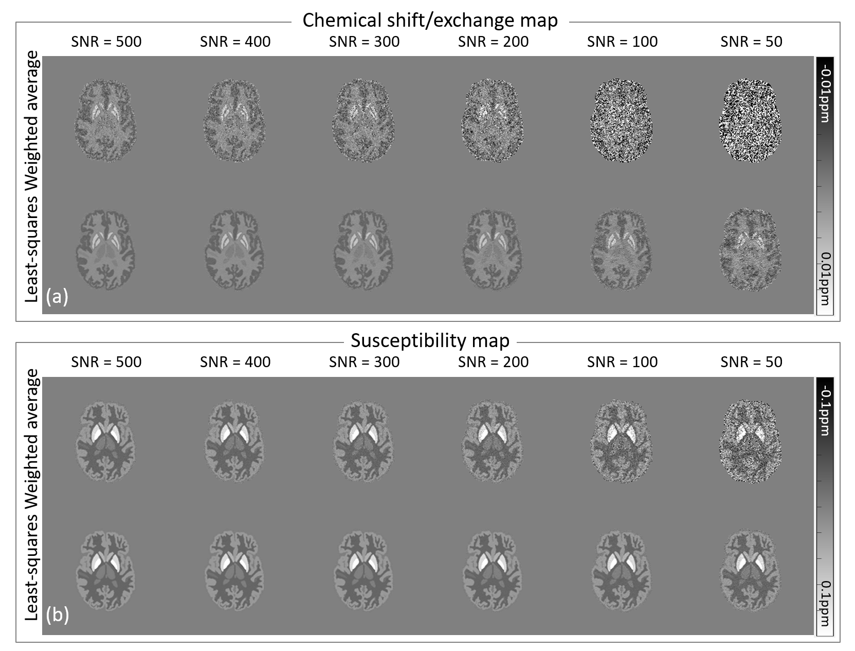
For the comparison of the noise amplification, magnitude values were assigned and Gaussian noise was added in both real and imaginary parts of the complex signal. Then, the complex images were generated for the SNR range from 50 to 500. The susceptibility and chemical shift/exchange maps were reconstructed using the two methods.
Another evaluation was performed to compare the condition number for various B₀ angles. For 6 and 12 directional data, one B₀ direction was oriented along the z-direction whereas the others were oriented uniformly in $$$\phi$$$ angles over $$$\mathrm{[0,2}\mathrm{\pi}\mathrm{)}$$$ with a fixed $$$\theta$$$ (Fig. 3a). The condition number was evaluated for $$$\theta$$$ from 1° to 90°.
[In-vivo application] Using twelve directional QSM challenge 2016 data⁹, we reconstructed both susceptibility and chemical shift/exchange maps by using the least-squares method.

Results

The proposed methods successfully reconstructed the susceptibility map and chemical shift/exchange map even for the small rotation angles (17.9 $$${\pm}$$$ 5.5°;12 directional data) in the noise-free condition (Figs. 1d and 1e). When the noise was added, the least-squares method showed more robust results than the weighted-average method (Fig. 2). When the condition number was explored, large condition numbers were observed for the angles smaller than 20° (6 and 12 directional data; Fig. 3). Figure 4 reported the in-vivo maps (12 directional data). The chemical shift/exchange map showed a smaller contrast range than the susceptibility map.

Conclusion and Disscussion

In this study, we proposed two methods that separate susceptibility and chemical shift/exchange in phase. Compared to the previous method that requires three orthogonal directional data, the proposed methods can utilize data with smaller head rotation. Still, multiple B₀ directions and large B₀ angle (e.g. 20° or larger for 6 directional data) are necessary. As a preliminary result, the chemical shift/exchange and susceptibility maps of the in-vivo human brain were generated. For a proper interpretation, however, further consideration is required for additional sources of frequency shift such as susceptibility anisotropy¹⁰ and microstructural anisotropy¹¹.

Acknowledgements

This work was supported by the National Research Foundation of Korea(NRF) grant funded by the Korea government(MSIT) (No. NRF-2018R1A2B3008445) and the Brain Korea 21 Plus Project in 2019.