Introduction

Quantitative susceptibility mapping (QSM) analysis enables to detect iron concentration and distribution from multi-echo phase images applied several complicated post-processing [1]. A similar iron evaluation has also been performed by the R2* relaxometry in the clinical setting, such as the brain and liver. However, it is well-known that R2* value depends on the temperature, which is the confounding factor of R2* measurement [2]. To clarify the temperature dependence of susceptibility estimated by QSM analysis, we investigated the relationships between temperature and susceptibility and R2* values using a simple cylinder phantom with varying temperatures.

Material and Methods

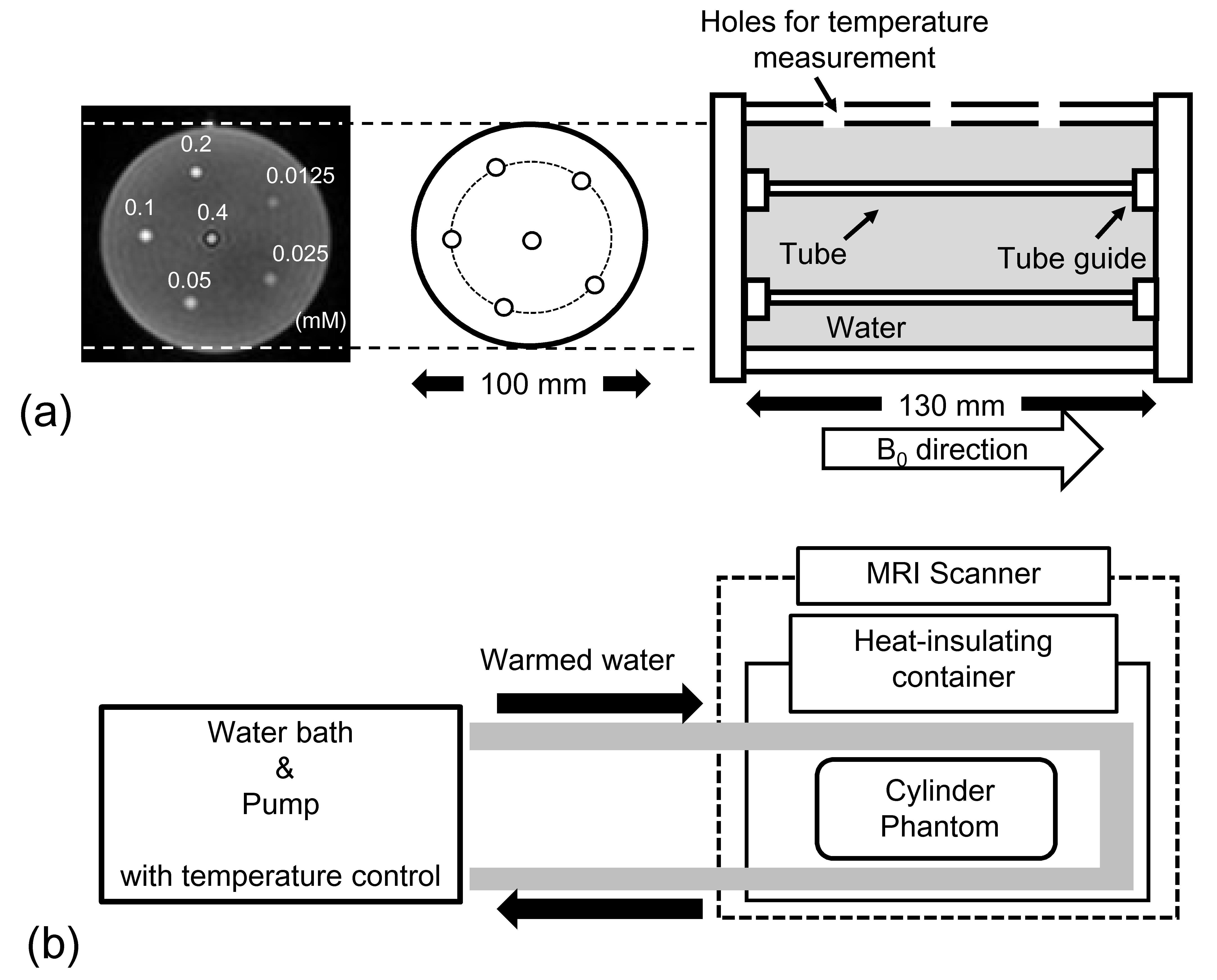
Phantom preparation
A schematic drawing of the cylinder phantom is shown in Fig. 1a. The six solutions with various concentrations of superparamagnetic iron oxide (SPIO) nanoparticles (0.0125, 0.025, 0.05, 0.1, 0.2, and 0.4 mM) were employed. The solutions were sealed to plastic tubes (φ = 6 mm, wall thickness = 0.05 mm). These tubes were placed in a cylinder phantom and were filled with water around to minimize the interaction in the air-water boundary. Fig. 1b illustrates the experimental setup of the phantom. The cylinder phantom was placed on an axis parallel to the magnetic field. The desired temperature water was circulated by the pomp around the cylinder phantom from the water bath with temperature control. The temperature of the circulated water was adjusted to change the temperature in the cylinder phantom to 25.8, 29.8, 31.6, 33.6, 35.6, 38.0, 40.0, and 42.5 ℃. The heat-insulated container was used to help maintain the temperature in the cylinder phantom. The water temperature during the examination was assured to measure the temperature by thermometer before and after every scan.

MRI experiment and data analysis
The cylinder phantom was scanned in the transverse plane with a 3T MRI (Hitachi Ltd., Tokyo, Japan). The magnitude and phase images were obtained using 3D multiple spoiled gradient echo sequence with the following parameters: FOV, 160 × 160 ×140 mm3; matrix size, 80 × 80 × 70 (zipped 160 × 160 × 140); TR, 32 ms; TE, 4.2-­27.4 ms at 2.9-ms intervals; number of echo, 9; and flip angle, 20°. The pre-scan was performed at every changing temperature. The local field was calculated from the multiple phase images by two-step background field removal, consisting of the Laplacian boundary value method [4] followed by iterative spherical mean value method [5] with the filter size of 5 mm. Next, the susceptibility map was estimated by the two-step non-linear morphology enabled dipole inversion algorithm [6] like a streaking artifact reduction for the QSM algorithm [7] to minimize the streaking artifact induced by high concentration solutions. The mean susceptibility of water in the cylinder phantom was used for zero reference of susceptibility. The R2* map was calculated from the magnitude images using auto-regression on linear operations algorithm [8]. The relationships between temperature and susceptibility and R2* values were determined. Moreover, the temperature coefficients of susceptibility (Tc-χ) and R2* (Tc-R2*) [2] from measurements at different temperatures were calculated at each concentration, and the linearities in these indices against the SPIO concentration were validated.

Results

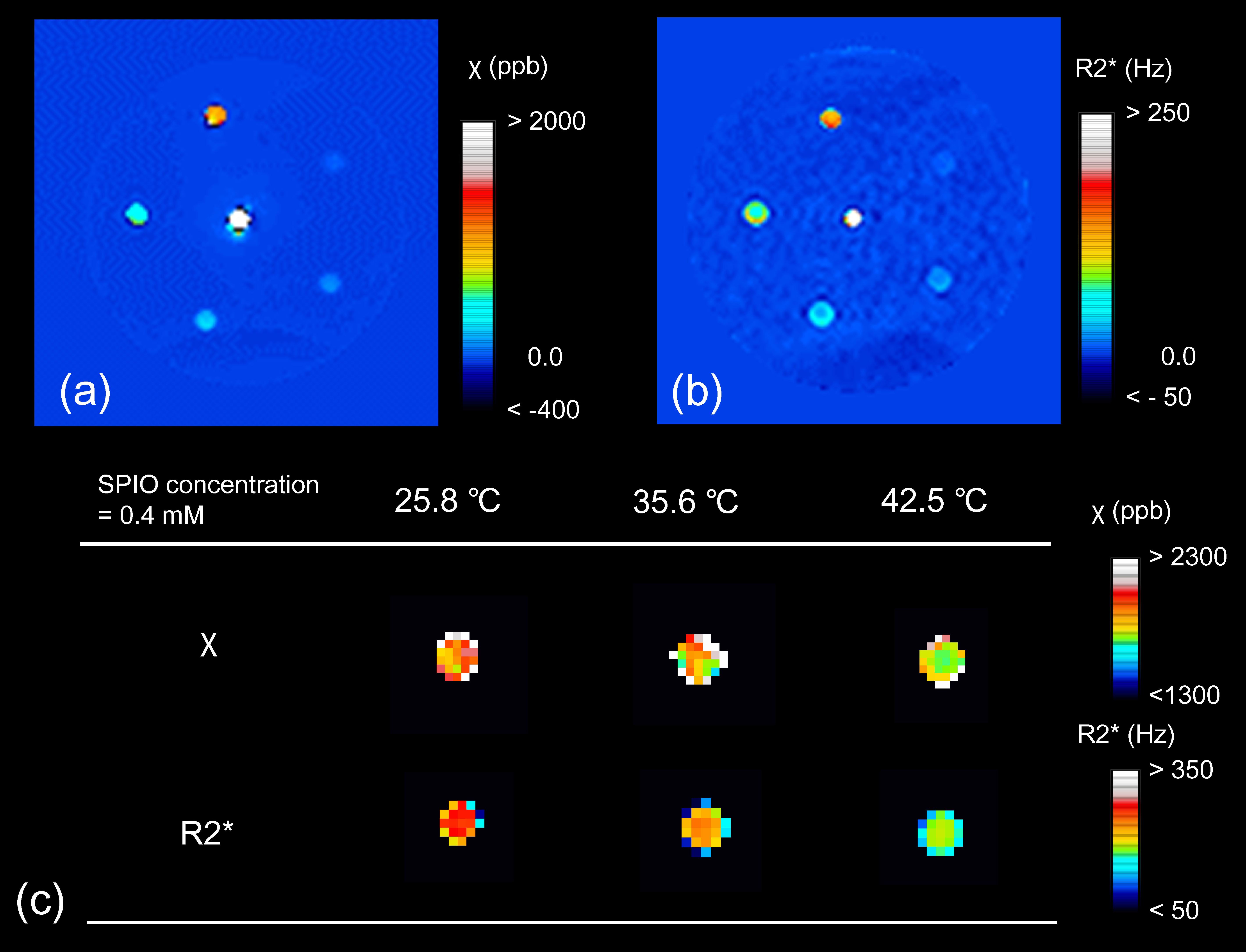
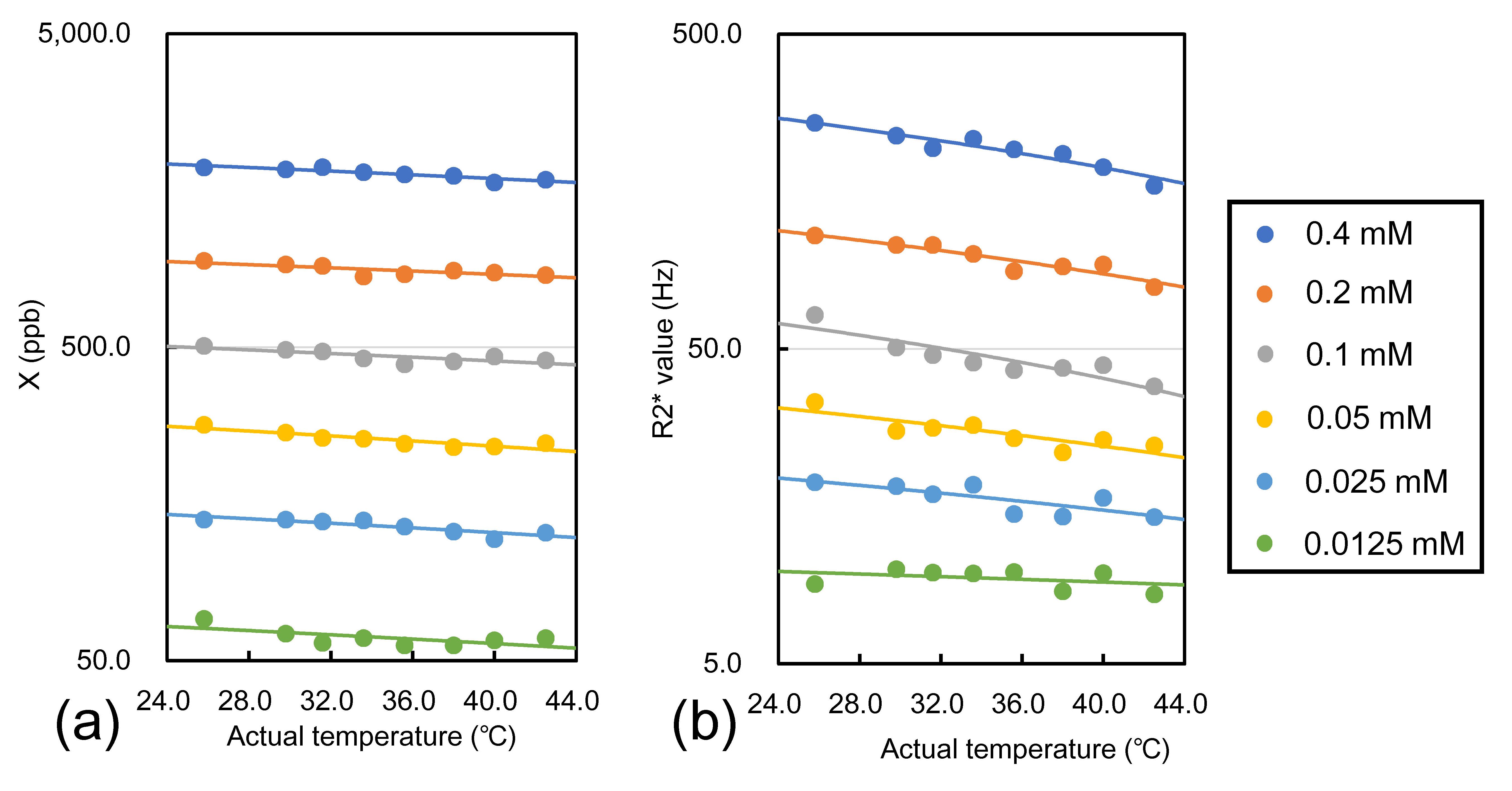
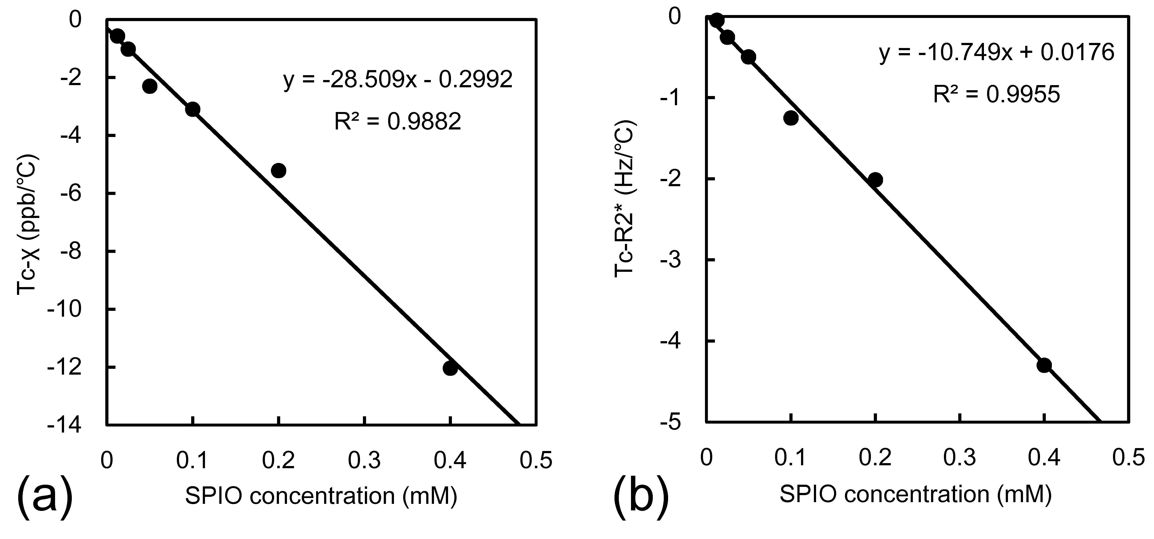
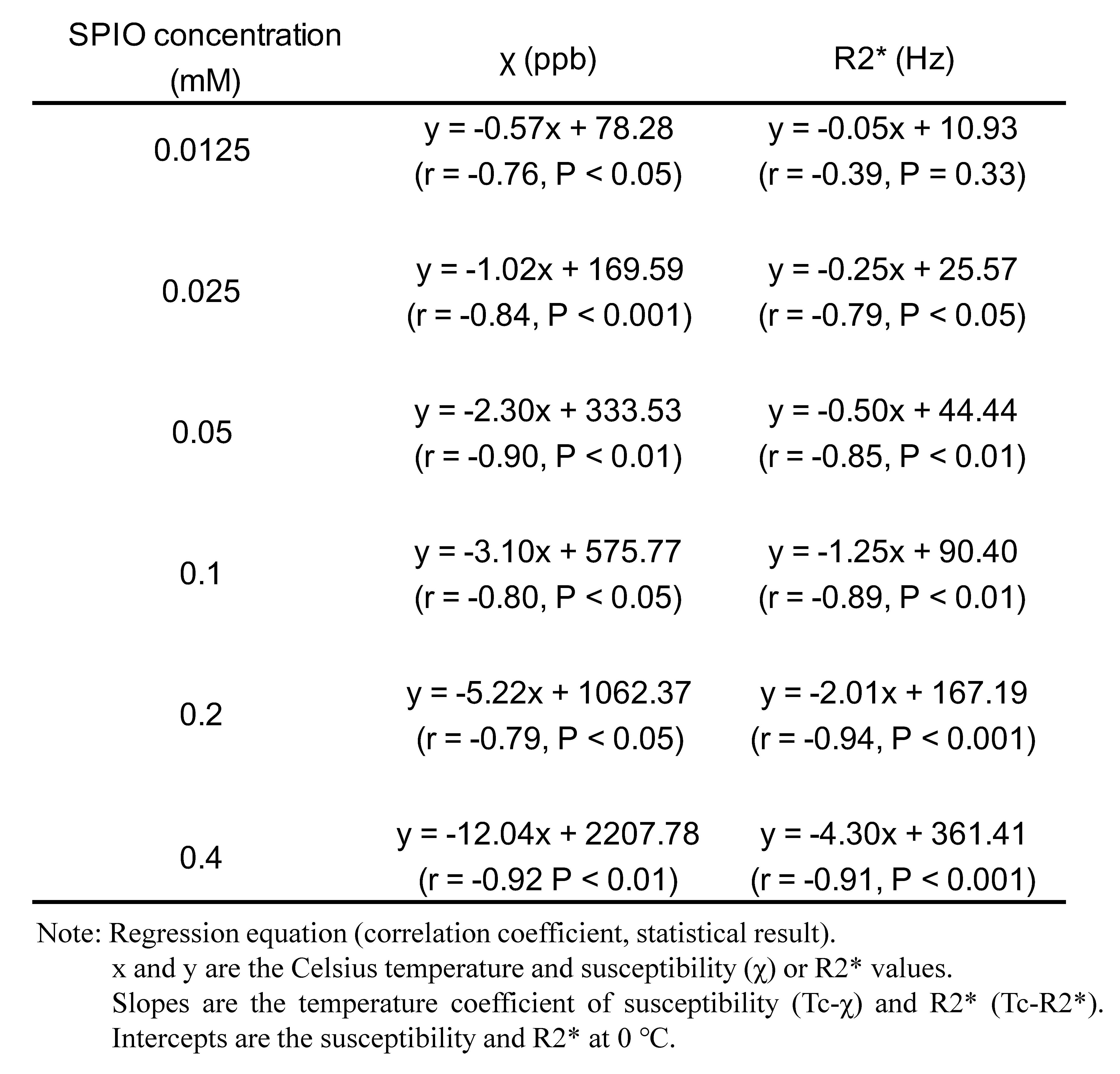
The resultant susceptibility and R2* maps in 25.8 ℃ are shown in Fig. 2a and b. Fig. 2c demonstrates that the susceptibility and R2* values at an SPIO concentration of 0.4 mM decreased with increasing temperature. There were clear temperature dependences of susceptibility and R2* values in each SPIO concentration (Fig.3). The significant inverse correlations were found between the temperature and susceptibility and R2* values at each SPIO concentration, except to 0.0125 mM in R2* (Table1). There were strong linearities between the SPIO concentration and Tc-χ (r = -0.99, P < 0.001) and Tc-R2* (r = -0.99, P < 0.001) (Fig. 4).

Discussions

It was successful in depicting the susceptibility of iron changed by the temperature using QSM analysis. The negative correlations between the susceptibility and R2* values can be explained by the decrease of paramagnetic iron susceptibility with increasing temperature based on Curie’s law [2, 8]. The susceptibility estimated by QSM analysis is a relative value based on proton resonance frequency (PRF) of water changed by the temperature [9]. However, the effect of the PRF shift of water to QSM analysis could be minimized by the use of water susceptibility in the cylinder phantom as zero reference in this study.
Moreover, Tc-χ and Tc-R2* linearly decreased with SPIO concentration. The volume susceptibility (χ) in a particular volume (V) considering the temperature is approximated as
$$\chi\approx\frac{\sum_{n=1}^k(\alpha_{n}T+\chi_{n, 0})V_{n}}{V}$$
where k is the number of particles, T is the Celsius temperature, α_n is the Tc-χ of particle n, V_n is the volume of particle n, and χ_n,0 is the susceptibility of particle n at 0 ℃. According to the above equation, the susceptibility in the voxel is proportional to the temperature and the number of particles (i.e., iron content in this study). Therefore, since the Tc-χ in the voxel varies considerably with the iron contents, the temperature might be the confounding factor of QSM-based iron estimation, similar to the R2* measurement.

Conclusion

There is a significant inverse correlation between the temperature and the susceptibility value estimated by QSM analysis. This dependence may be the confounding factor of the QSM-based iron estimation.

Acknowledgements

This work was supported by JSPS KAKENHI Grant Number JP17K15805.