3202
U3-Net for Deep Vector QSM – Solving the Susceptibility Tensor Phase Model in Single-Orientation MRI1Buffalo Neuroimaging Analysis Center, Department of Neurology at the Jacobs School of Medicine and Biomedical Sciences, University at Buffalo, The State University of New York, Buffalo, NY, United States, 2Department of Computer Science and Automation, Technische Universität Ilmenau, Ilmenau, Germany, 3Center for Biomedical Imaging, Clinical and Translational Science Institute, University at Buffalo, The State University of New York, Buffalo, NY, United States
Synopsis
Quantitative susceptibility mapping (QSM) is increasingly being used to study the brain iron homeostasis and white matter pathology. However, all QSM algorithms that are currently used in the clinical setting use a physical model that neglects the well-established anisotropic magnetic susceptibility of myelin. In this work, we demonstrate that an extended U-Net allows solving a Vector QSM model that accounts for field perturbations caused by off-diagonal tensor elements. The proposed Deep Vector QSM yielded improved estimates of χ33 compared to conventional QSM.
Introduction
Quantitative susceptibility mapping (QSM)1 is increasingly being used to study the brain iron homeostasis and white matter pathology. All clinically-used QSM algorithms calculate a single (scalar) susceptibility value $$$\chi$$$ per voxel, assuming that tissue susceptibility is isotropic ($$$d$$$: unit dipole; $$$\Delta B$$$: field perturbation; $$$\star$$$: convolution):2$$\Delta B= \chi \star d \text{. (1)}$$
The well-established anisotropic magnetic susceptibility of myelin3 renders this assumption invalid in the white matter. Using the rank-2 susceptibility tensor and assuming $$$B=B_0 \cdot (0,0,1)^T$$$, the field perturbation is given by the three tensor elements $$$\chi_{13}$$$, $$$\chi_{23}$$$, and $$$\chi_{33}$$$:4
$$\Delta B= \chi_{13} \star d_{13} + \chi_{23} \star d_{23} + \chi_{33} \star d_{33} \text{. (2)}$$
Here, $$$d_{33}=d$$$, and $$$d_{13}$$$ and $$$d_{23}$$$ are the specific unit response functions for the off-diagonal tensor elements $$$\chi_{13}$$$ and $$$\chi_{23}$$$, respectively. The 2016 QSM Reconstruction Challenge demonstrated that ignoring the additional terms introduces artifacts in susceptibility maps.4 While Susceptibility Tensor Imaging (STI)5 can measure the complete tensor, its requirement of at least six head orientations renders the technique clinically infeasible. Liu et al.6 have proposed solving Eq. (2) with an algorithm similar to the MEDI approach7. In this work, we demonstrate that an extended U-Net allows solving Eq. (2). The proposed Deep Vector QSM yielded improved estimates of $$$\chi_{33}$$$ compared to conventional QSM.
Methods
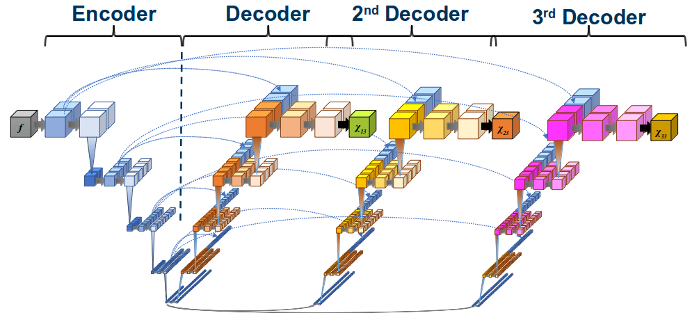
Network architecture and training: We extended Jochmann et al.’s generalized U-Net architecture8,9 by a third decoder arm (Fig. 1) and trained the network (Tensorflow v2.0; NVidia-GeForce-2080Ti) using synthetic maps of $$$\chi_{13}$$$, $$$\chi_{23}$$$ and $$$\chi_{33}$$$ at the output nodes and field maps simulated according to Eq. (2) at the input nodes. We used 2400 training and 600 validation data sets as described previously (96x96x96).8 To increase the robustness of the network to noise and different ranges of susceptibility values, we added Gaussian noise to the field maps and included scaling-based data augmentation.Conventional QSM: For comparison of the proposed technique (Eq. 2) with conventional DeepQSM10 (Eq. 1), we trained a U-Net with only $$$\chi_{33}$$$ and field maps simulated according to Eq. (1).
Evaluation: We applied both techniques to the 2016 QSM Reconstruction Challenge dataset4 and compared results to the provided gold-standard STI dataset.
Results
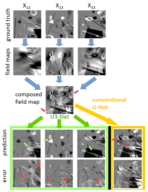
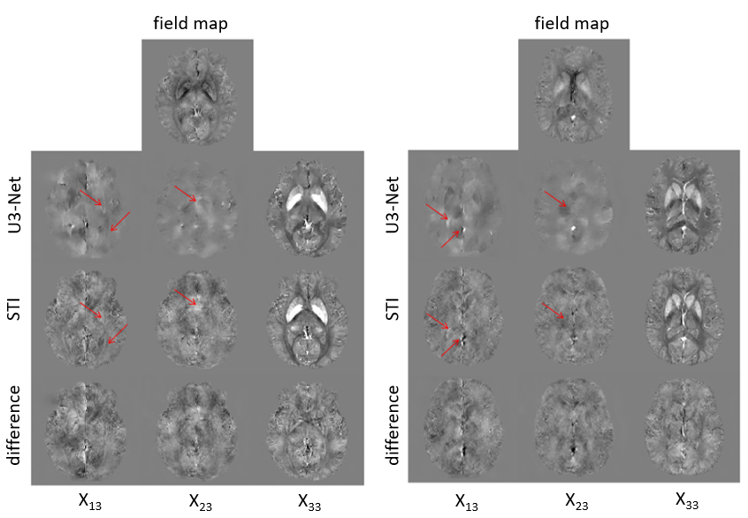
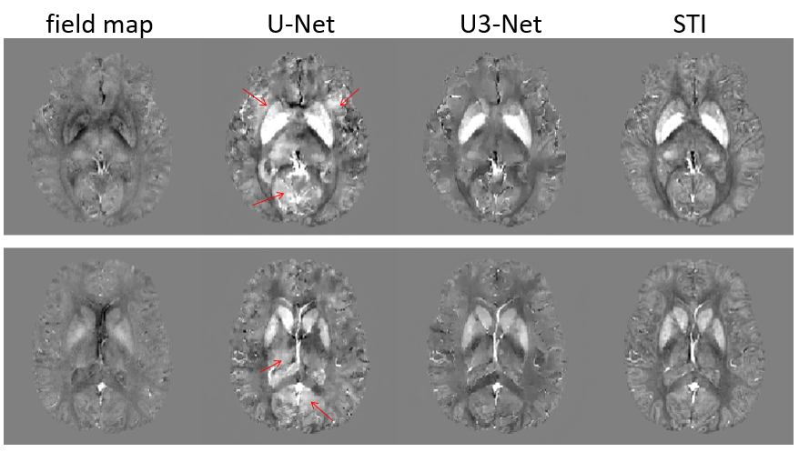
Application of Deep Vector QSM to the validation data demonstrated disentanglement of tensor elements that had a measurable effect on the field map (Fig. 2). Inaccuracies occured when an object was hardly visible in the magnetic field and when objects had more than one non-zero tensor component at the same time. The prediction of DeepQSM included objects that belonged to the $$$\chi_{13}$$$ and $$$\chi_{23}$$$ source maps. The $$$\chi_{33}$$$ maps of Deep Vector QSM and STI were highly similar and did not show apparent artifacts (Fig. 3). Reconstruction quality was substantially improved compared to the map obtained with DeepQSM (U1-Net) from the same field-map (Fig. 4). The $$$\chi_{13}$$$ and $$$\chi_{23}$$$ maps demonstrated shared features using Deep Vector QSM or STI (Fig. 3-arrows).Discussion
We demonstrated the feasibility of solving the Vector QSM problem (Eq. 2) using an extended U-Net architecture. While the cross-diagonal tensor terms showed only few anatomical features in both VectorQSM and STI, the extended physical model improved the $$$\chi_{33}$$$ map compared to conventional QSM. The disentanglement of all three tensor elements from a single field map is likely enabled by the different mathematical structure of the three convolution kernels in Eq. (2). Future work will focus on improved synthetic training data to further improve the reconstruction quality in vivo.Conclusion
Deep neural networks enable the solution of more realistic physical models for quantitative phase MRI. The improved estimation of tissue susceptibility in the white matter will bring us one step closer to a reliable application of QSM in the white matter.Acknowledgements
Research reported in this publication was funded by the German Academic Exchange Agency (DAAD) Rise Worldwide program and the National Center for Advancing Translational Sciences of the National Institutes of Health under Award Number UL1TR001412. The content is solely the responsibility of the authors and does not necessarily represent the official views of the NIH of DAAD.References
1. Reichenbach JR et al. Quantitative Susceptibility Mapping: Concepts and Applications. Clin Neuroradiol 2015, 25(S2):225–30.
2. Schweser et al. Foundations of MRI phase imaging and processing for Quantitative Susceptibility Mapping (QSM). Z Med Phys 2016, 26(1):6–34.
3. Li W et al. Susceptibility Tensor Imaging (STI) of the Brain: Review of Susceptibility Tensor Imaging of the Brain. NMR Biomed 2017, 30(4):e3540.
4. Langkammer C et al. Quantitative susceptibility mapping: Report from the 2016 reconstruction challenge. Magn Reson Med 2018. 79(3): 1661–73.
5. Liu, C. Susceptibility tensor imaging. Magn Reson Med 2010, 63(6):1471-1477.
6. Liu, T et al. Vector Model for Quantitative Susceptibility Mapping (Vector QSM). ISMRM 2015, p928.
7. Liu J. Morphology enabled dipole inversion for quantitative susceptibility mapping using structural consistency between the magnitude image and the susceptibility map. Neuroimage. 2012;59(3):2560–2568.
8. Jochmann T et al. U2-Net for DEEPOLE QUASAR–A Physics-Informed Deep Convolutional Neural Network that Disentangles MRI Phase Contrast Mechanisms. ISMRM 2019, p320.
9. Ronneberger O, Fischer P, Brox T. U-Net: Convolutional Networks for Biomedical Image Segmentation. arXiv:1505.04597 [cs] 2015.
10. Bollmann et al. DeepQSM - Using Deep Learning to Solve the Dipole Inversion for Quantitative Susceptibility Mapping. NeuroImage 2019, 195:373-383.
Figures