Introduction

The variational minimization problem for the ill-posed dipole inversion in susceptibility mapping is given by: $$\text{argmin}_{\chi}\frac{\mu}{2}||D\chi - \varphi||_2^2+R(\chi)$$ where $$$\chi$$$ is the magnetic susceptibility, $$$D$$$ is the dipole convolution matrix, $$$\varphi$$$ the local field, and $$$R(\cdot)$$$ a regularizer. Equation [1] can be solved using a proximal gradient descent (PGD) method: $$\chi_{k+1}=\text{prox}_{R}(\chi_k-\tau_{k}D^*(D\chi-\varphi))$$ where the proximal operator prox depends on $$$R$$$. Mardani et al. proposed to learn the proximal operator using residual networks for 2D undersampled compressed sensing image reconstruction¹. We adopt this strategy of learning the proximal operator for the dipole inversion, but due to memory constraints inherent to 3D problems, we have to adjust the neural network architecture. Given a zero initial input $$$\chi_0$$$, unrolling the first two iterations of the above iterative scheme yields: $$\chi_1=\text{prox}_1(D^*\varphi)$$ $$\chi_2=\text{prox}_{2}(\chi_1-\tau_{2}D^*(D\chi-\varphi))$$ where we absorbed $$$\tau_1$$$ into the first proximal operator. Ignoring the second prox operator temporarily, we are left with $$$D^*\varphi$$$ as input into a neural network whose output is passed into a single gradient descent step. As multiple iterations are increasingly memory intensive we propose to maximize the capacity of the neural network in the first step and only use the first two iterations of the learned PGD. To do so, we choose the V-Net architecture². We demonstrate that V-Net alone outperforms the U-Net³-based QSMnet⁴ model. Then, we improve the V-Net model by combining the physics of the dipole problem with the expressive power of the V-Net; the proposed ProxVNET model is trained utilizing the iteration scheme in Equation [3].

Methods

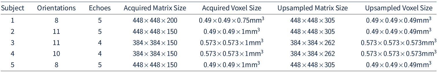
Data acquisition High-resolution 3D-GRE data was acquired from 5 healthy volunteers, with 12 multiple-echo scans at varying head orientations on a Philips Achieva 3T scanner. Images were upsampled to isotropic resolution by zero-filling in the Fourier domain. Quality assurance inspection was performed on each scan in order to check for motional and foldover artifacts. A total of 48(=8+11+11+10+8) multiple-echo scans remained, with subject #4 (10x4=40 3D images) used for testing, and the remaining 4 subjects (11x4+(8+11+8)x5=179 3D images) used for training and validation. The scan parameters for all 5 datasets are summarized in Table 1. For each volunteer, the multiple-orientation reference COSMOS was computed for each echo using all remaining scan orientations. Each echo was unwrapped using Laplacian unwrapping⁵; the background field was removed using v-SHARP⁶; NiftyReg was used with default parameters to register the scans to the neutral frame⁷. These COSMOS reconstructions were then used as the target susceptibility maps during training and testing.
Network architecture For the proximal operator in the first iteration we use a V-Net with pre-activation (BatchNorm + ReLu) convolutional layers with 3x3x3 filters. We further incorporate a single pre-activation residual block after the first convolutional layer (before downsampling) and in front of the very last 1x1x1 convolutional layer. A skip connection between the input and output was added for residual learning. For the second proximal operator we use a 7x7x7x1x32 convolutional layer followed by a 3x3x3 convolutional layer + ReLu, another 3x3x3 convolutional layer without activation and finally a 1x1x1 convolutional layer. Networks were trained on 64x64x64 patches. Training data was generated by randomly sampling 100 patches from each of the 179, multi-orientation, multi-echo, multi-resolution images. Adam with decoupled weight decay (AdamW)⁸ was used to train the network, with a constant learning rate of 3e-4 and weight decay of 1e-5. The $$$\ell_1$$$ loss function was used. No further data augmentation was performed. Batch size used was 8. The network was implemented using the Julia programming language. All networks were trained using the same training data and optimization algorithm + parameters on a NVIDIA Quadro P6000 GPU with 24GB of memory.

Results

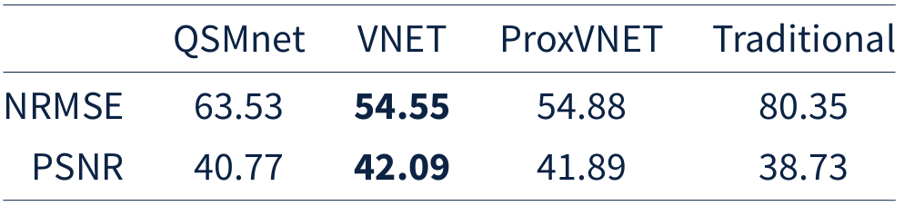
Both V-Net and ProxVNET outperform our in-house LSMR-based dipole inversion algorithm⁹ as well as QSMnet, as seen Table 2. V-Net and ProxVNET perform similarly well. Figure 1 shows higher visual reconstruction quality for V-Net and ProxVNET compared to QSMnet, as well.

Discussion and Conclusion

In this work we proposed a deep learning model, ProxVNET, in order to solve the ill-posed dipole inversion in susceptibily mapping. ProxVNET is derived from unrolled proximal gradient descent iterations wherein the proximal operator is a learned V-Net. Both V-Net and ProxVNET outperform the U-Net-based dipole inversion deep learning model QSMnet when compared to the COSMOS reconstructed susceptibility maps.

Acknowledgements

Natural Sciences and Engineering Research Council of Canada, Grant/Award Number 016-05371 and the Canadian Institutes of Health Research, Grant Number RN382474-418628.