Purpose

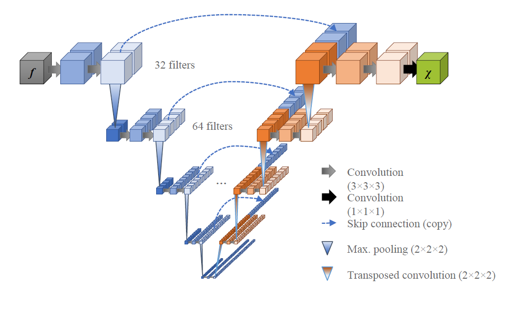
Deep convolutional neural networks have recently gained popularity for solving the ill-posed dipole inversion problem in Quantitative Suscep-tibility Mapping (QSM).¹ At the same time, the recent 2019 QSM reconstruction challenge has seen many deep-learning-based submissions far behind classical methods, many of them using the same U-Net architecture² (see Fig. 1).
A U-Net, originally developed for image segmentation, is suitable for solving a wide range of ill-posed problems³ and it is the training data that defines what function it approximates. The physical fidelity and the capability to generalize to real-world applications depends on the quality of the training data.
For QSM, the neural networks are used to approximate the inverse mapping from the Larmor frequency $$$f$$$ to the magnetic susceptibility $$$\chi$$$. The training of the neural networks is performed with examples of $$$\chi$$$ and $$$f$$$ that can either be obtained from physical simulations on synthetic source distributions⁴ or through “classical” QSM methods on real data, potentially using additional information, for example using COSMOS.⁵ For both choices, there are a plethora of decisions to make and parameters to set. Here we seek to present best practices regarding the modeling of synthetic source distributions and data augmentation.

Methods

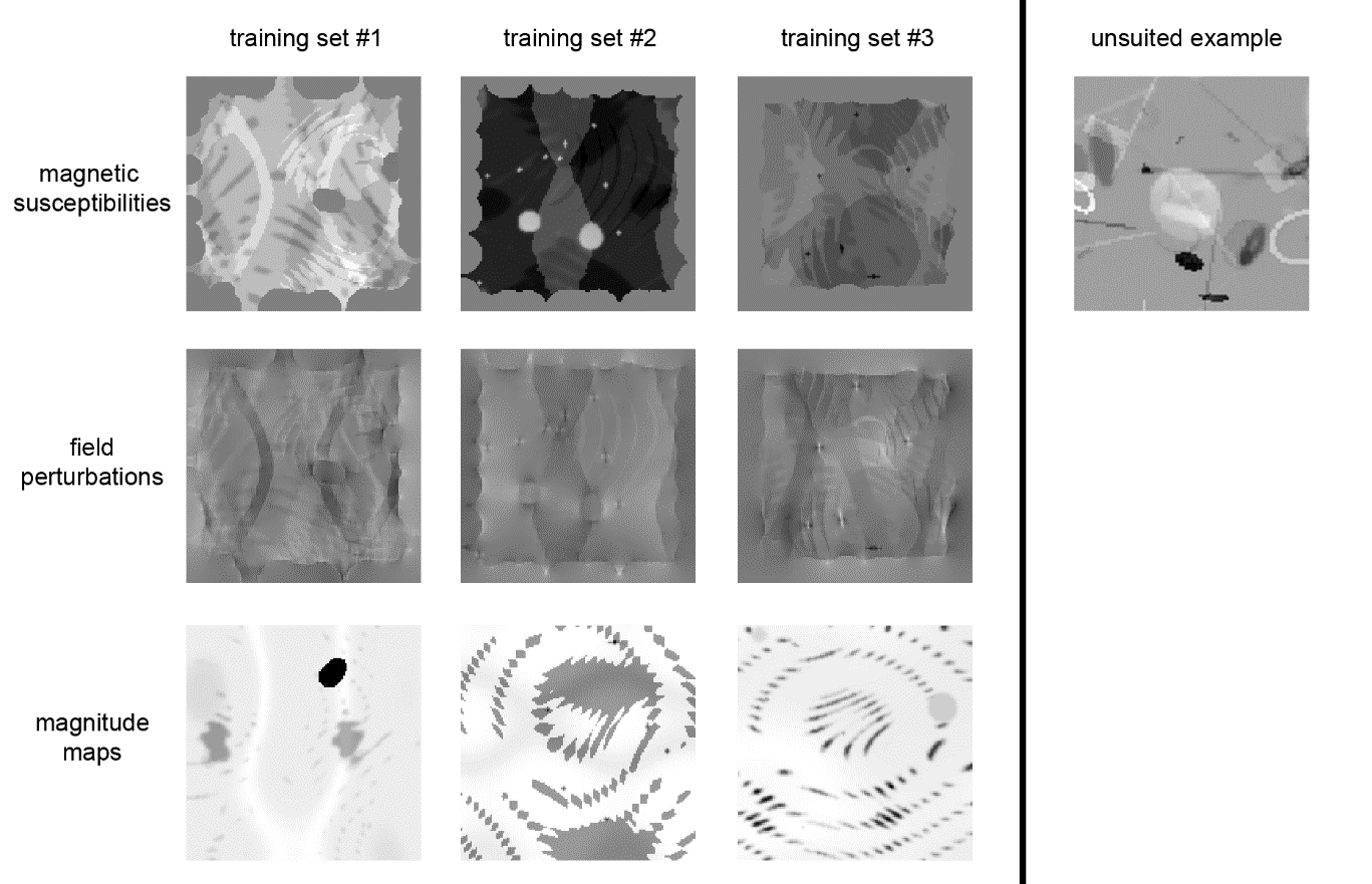
Network Architecture: We set up a U-Net with 3-dimensional in- and output layers (Tensorflow 2.0).
Physics-informed training: We used syn-thetic, entirely non-anatomical data for the training of the network weights because of the uncertain ground truth in real data, the scarcity of available datasets, and to preclude anatomical bias. We generated $$$N=1320$$$ source distributions of $$$\chi$$$ by randomly placing (differently smoothed) objects in a volume of $$$144^3$$$ voxels and simulated $$$f$$$ from the generated $$$\chi$$$ via Fast Forward Field Computation.⁶ We trained for 500 epochs with ADAM, augmenting the full training set between epochs by randomly rotating (90° steps along the z-axis), flipping (x, y, z) and scaling the values (factors 0.1 to 2) as well as adding Rician noise. To balance the learning from down-scaled and up-scaled examples, a tailored loss function was required, as the common loss metrics for gradient descent, such as mean squared error, are not invariant against scaling. Thus, we introduce the following loss function:
$$L=\left\lVert f_\mathrm{ground truth} - f_\mathrm{prediction} \right\rVert^2 / \mathrm{variance}(f_\mathrm{ground truth}).$$
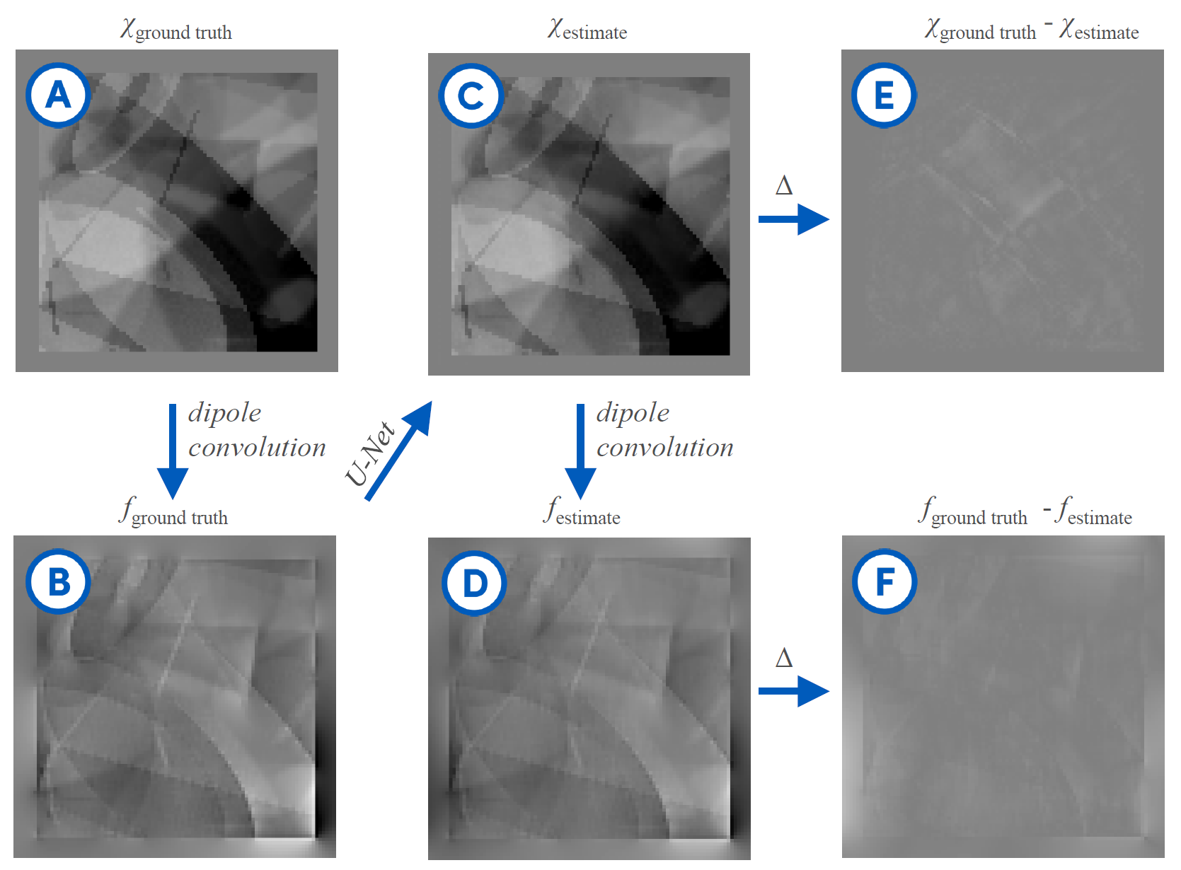
Evaluation: To evaluate the algorithm in silico, we assessed the differences between the predictions of $$$\chi$$$ and their ground truth patterns. Furthermore, we used the datasets from the 2019 QSM Reconstruction Challenge to evaluate the algorithm on a realistic human brain model.

Results and Discussion

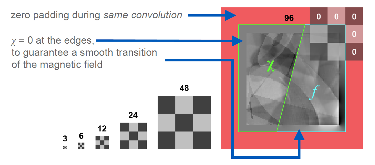
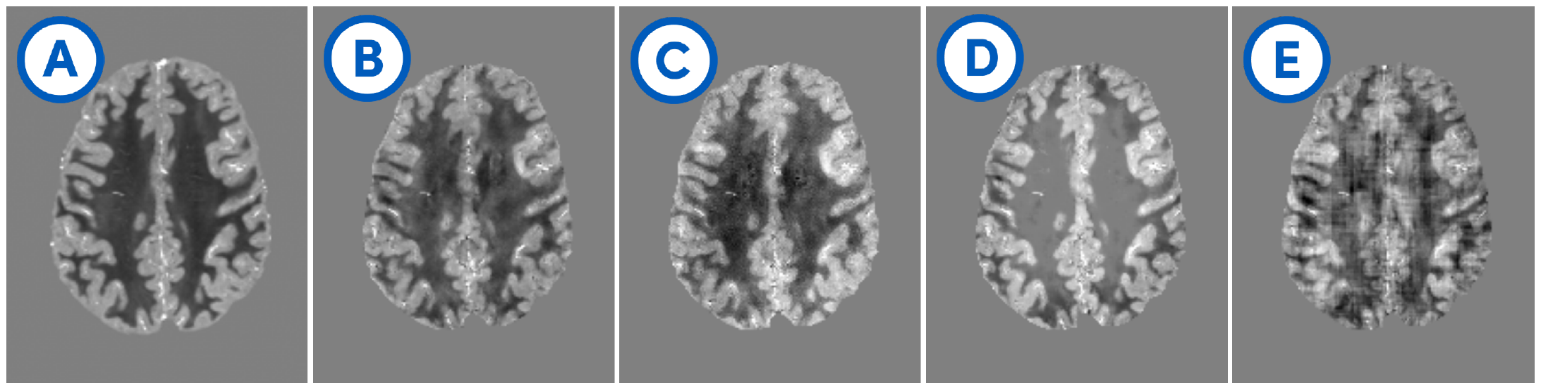
Our synthetic evaluation patterns were reconstructed to a degree that made them almost indistinguishable from the ground truth (see Fig. 2). The assessment on the reconstruction challenge dataset revealed that different variants of the training data imposed different shortcomings that each needed to be addressed. First, there were strong inhomogeneities in the white matter that required filling the training volumes with more non-zero regions. Then, there were block-shaped artifacts that could be mitigated by leaving space at the edges of the source volumes to allow the corresponding field to decay within the volume, and hence ensure consistency of the physical model at the edges of the volume. Adding simulated Rician noise to the field distributions successfully suppressed noise amplification in the susceptibility estimates.
It was important to have many and diverse training patterns to cover a wide range of local scenarios, meaning susceptibility gradients and steps in any direction. Different representations of the dipole (declaration in the spatial or Fourier domain) had only a negligible impact. Flipping, rotating and scaling the training samples between epochs to increase the effective training data size strongly improved the mapping as measured by the mean squared error on the reconstruction of the synthetic evaluation set.
We expected 16 kernels in the first layer to be too few because the detection of edges in 45-degree steps in three dimensions already requires 26 kernels when using a rectifying activation function. Further kernels are needed to sense average values and fine, pixel-sized structures. Indeed, we found 32 kernels to perform better, while our networks did not make use of the potentially higher capacity of 48 or 64 kernels.
While the original U-Net crops the data from layer to layer and outputs a much smaller image, we opted for zero-padding to allow for an output size identical to the input size. This requires to set the source distributions close to the borders to zero. The reason is, that magnetic susceptibility at the edges of a volume cause non-zero field distortions beyond the volume’s border, hence, zero-padding would introduce false physical examples that leads to artifacts in the reconstruction (see Fig. 2).

Conclusion

We presented a simulation and training strategy with physics-aware augmentation and a custom loss function to train a deep convolutional neural network for QSM.

Acknowledgements

Research reported in this publication was funded by the National Center for Advancing Translational Sciences of the National Institutes of Health under Award Number UL1TR001412. The content is solely the responsibility of the authors and does not necessarily represent the official views of the NIH.