3193

On the usage of deep neural networks as a tensor-to-tensor translation between MR measurements and electrical properties

Ilias Giannakopoulos^1,2, José Serallés², Georgy Guryev^1,2, Luca Daniel², Elfar Adalsteinsson^2,3, Lawrence Wald^4,5,6, Daniel Sodickson^7,8,9, Jacob White², and Riccardo Lattanzi^7,8,9
¹Skoltech Center for Computational and Data-Intensive Science and Engineering, Skolkovo Institute of Science and Technology, Moscow, Russian Federation, ²Department of Electrical Engineering & Computer Science, Massachusetts Institute of Technology, Cambridge, MA, United States, ³Institute for Medical Engineering and Science, Cambridge, MA, United States, ⁴Department of Radiology, Massachusetts General Hospital, Charlestown, MA, United States, ⁵Department of Radiology, Harvard Medical School, Boston, MA, United States, ⁶Harvard-MIT Health Sciences and Technology, Cambridge, MA, United States, ⁷Center for Advanced Imaging Innovation and Research (CAI2R), Department of Radiology, New York University School of Medicine, New York, NY, United States, ⁸The Bernard and Irene Schwartz Center for Biomedical Imaging (CBI), Department of Radiology, New York University School of Medicine, New York, NY, United States, ⁹Sackler Institute of Graduate Biomedical Sciences, New York University School of Medicine, New York, NY, United States

Synopsis

Electrical properties (EP) can be retrieved from magnetic resonance measurements. We employed numerical simulations to investigate the use of convolutional neural networks (CNN) as a tensor-to-tensor translation between transmit magnetic field pattern ($$$b_1^+$$$) and EP distribution for simple tissue-mimicking phantoms. Given the volumetric nature of the problem, we chose a 3D UNET and trained the network on $$$10000$$$ data. We investigated on the usage of regularization to account for overfitting and observed that multiple dropouts through the layers of the network yield optimal EP reconstructions for $$$1000$$$ testing data.

Introduction

Frequencies in high-field scanners are high enough, and the associated wavelengths in tissue short enough, that it is becoming tractable to solve the inverse scattering problem associated with estimating tissue electrical properties from $$$b_1^+$$$ measurements (electrical property tomography). Methods based on local field or phase gradients (e.g. LMT) have met with some success, though their sensitivity to noise has proved problematic^1,2. Global optimization-based methods (e.g. GMT) are less sensitive to noise, but are extremely computational expensive³. In this paper we describe our experiments with using multi layer neural networks to represent the map from $$$b_1^+$$$ measurements to tissue electrical properties (EP). And since neural networks require large data sets for training, we take advantage of tools like MARIE 2.0⁴, which can quickly and accurately compute volume fields given tissue and coil properties, and thus enable the generation of virtual data sets exhaustive enough for training.

Theory and Methods

We generated a dataset of $$$11000$$$ scatterers enclosed by an $$$8$$$-channel transmit-receive triangular coil⁵ (Figure 1) using the MARIE 2.0 electromagnetic field solver. All data points were enclosed in a cuboid domain of dimensions $$$8.8\times 8.8 \times 12.8 \text{cm}^3$$$, and the shape varied between a homogeneous cylinder, cuboid, or ellipsoid with random size and different tissue-mimicking properties. Inside each scatterer we inserted between $$$3$$$ to $$$12$$$ spherical features with arbitrary dimensions and random tissue-mimicking properties to introduce inhomogeneity. The voxel isotropic resolution was $$$4 \text{mm}$$$, and each scatterer was excited with one channel of the coil at a time, which resulted in inhomogeneous $$$b_1^+$$$ maps⁶ (the coil was tuned, matched and decoupled while loaded with a homogeneous cylinder). The input of the network was a $$$15$$$ channel tensor, which consisted of the absolute value of the $$$b_1^+$$$ for each of the $$$8$$$ channels and the $$$7$$$ relative phases between each channel and the first one, for each voxel of the scatterer. The output was a $$$2$$$ channel tensor, where each channel represented the relative permittivity $$$(\epsilon_r)$$$ and the conductivity $$$(\sigma_e)$$$, respectively. Given that the inverse problem is intrinsically 3D, the network of choice was a 3D UNET⁷ which is detailed in Figure 2. The size of each individual layer’s channel is shown above the schematics. The choice of a $$$3 \times 3 \times 3$$$ convolutional kernel is used to account for the strong local interactions between the $$$b_1^+$$$ and the EP. A hidden layer with the same kernel was inserted after the first layer to enlarge this region to $$$6 \times 6 \times 6$$$ voxels. The network consists of an analysis and a synthesis step. In the analysis, after down-sampling with max pooling we double the size of the channels, while in the synthesis we halve them after each transpose convolution.

Results

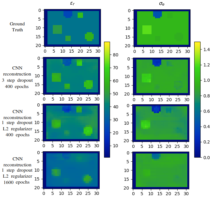
For the training process, we used the mean squared error (MSE) between reconstructed and true EP as the cost-function and applied the Adam solver with learning rate $$$0.0002$$$ and momentum parameters $$$0.5$$$ and $$$0.999$$$. The Rectified Linear Units in the synthesis were leaky with slope $$$0.2$$$, while in the analysis layers were not leaky. For the regularization, we cross-validated on various cases, and we observed that dropout with rate of $$$0.1$$$, $$$0.25$$$ and $$$0.5$$$ applied to the second, third and final level of both analysis and synthesis steps is the most optimal choice to account for overfitting and fast training. We trained the network on $$$10000$$$ noise-free data, with batch size of $$$4$$$, and tested on the remaining $$$1000$$$. The training loss is shown in Figure 3 (left) for $$$400$$$ epochs. The histogram of the MSE for all testing examples and all voxels of the domain, is shown in Figure 3 (right). In Figure 4 (left) we show the reconstructed EP, for the middle sagittal slice, for two representative, noise-free, testing examples. In Figure 4 (right) we show the performance of the network, after corrupting the $$$b_1^+$$$ of a testing example with Gaussian noise of peak signal-to-noise ratio (SNR) of $$$200$$$, $$$150$$$ and $$$100$$$ respectively. Specifically, the network performs well for high SNR, but for values around $$$100$$$ it treats the noise as a different $$$b_1^+$$$. In Figure 5 we compare the three steps dropout regularizer with a combination of an $$$L_2$$$ regularizer of weight $$$0.0001$$$ added on the cost-function and a dropout of rate $$$0.5$$$ applied only on the fourth step. The effect of $$$L_2$$$ regularizer smooths the reconstruction as expected and as a result some spherical features are not detected, even if we train for a higher number of epochs.

Discussion and Conclusions

The proposed UNET can model the relation between the EP and measurable MR measurements for simple tissue-mimicking phantoms and a specific excitation. The proposed CNN could be used on its own or in tandem with GMT, as a fast generator of a reasonable initial guess to considerably reduce the required number of iterations of the optimizer. In addition, one can use such network for the forward problem using the EP as an input and an electromagnetic field-related measurement as an output. Future work will investigate more robust network architectures, data generation and training for heterogeneous head models and performance in the presence of noise⁸.

Acknowledgements

This work was supported in part by grants from the Skoltech-MIT Next Generation Program and by grant NSF 1453675 from the National Science Foundation.

References

[1] van Lier, Astrid LHMW, et al. "Electrical properties tomography in the human brain at 1.5, 3, and 7T: a comparison study." Magnetic resonance in medicine 71.1 (2014): 354-363.

[2] Sodickson, Daniel K., et al. "Local Maxwell tomography using transmit-receive coil arrays for contact-free mapping of tissue electrical properties and determination of absolute RF phase." Proceedings of the 20th Annual Meeting of ISMRM. Concord, California, USA: ISMRM, 2012.

[3] Serallés, José EC, et al. "Noninvasive Estimation of Electrical Properties from Magnetic Resonance Measurements via Global Maxwell Tomography and Match Regularization." IEEE Transactions on Biomedical Engineering (2019).

[4] Guryev, G. D., et al. "Fast field analysis for complex coils and metal implants in MARIE 2.0." ISMRM (2019)

[5] Chen, Gang, et al. "A highly decoupled transmit–receive array design with triangular elements at 7 T." Magnetic resonance in medicine 80.5 (2018): 2267-2274.

[6] Giannakopoulos, Ilias I., et al. "Global Maxwell Tomography using an 8-channel radiofrequency coil: simulation results for a tissue-mimicking phantom at 7T." 2019 IEEE International Symposium on Antennas and Propagation and USNC-URSI Radio Science Meeting. IEEE, 2019.

[7] Çiçek, Özgün, et al. "3D U-Net: learning dense volumetric segmentation from sparse annotation." International conference on medical image computing and computer-assisted intervention. Springer, Cham, 2016.

[8] Isaev, Igor, and Sergey Dolenko. "Training with Noise Addition in Neural Network Solution of Inverse Problems: Procedures for Selection of the Optimal Network." Procedia computer science 123 (2018): 171-176.

Figures

Figure 1: Domain of interest that encloses all possible scatterers of choice (homogeneous cylinders, ellipsoids and cuboids with random dimensions and $$$3$$$ to $$$12$$$ spherical features with different EP). The scatterer loads an $$$8$$$ channel radiofrequency coil. The working frequency was $$$297.2$$$ MHz, corresponding to $$$7$$$ Tesla MRI.

Figure 2: 3D UNET. On the left the table denotes the operations through the hidden layers of the network and on the top the number of the channels is shown for each layer. Each operation is followed by appropriate padding and dilation sizes to keep the dimensions consistent.

Figure 3: (left) Sum of mean squared errors for all training examples. An error close to $$$2\%$$$ indicates good training, without overfitting. (right) Histogram of the MSE for both the relative permittivity and the conductivity for all $$$1000$$$ testing examples. The error remains small between $$$0\%$$$ and $$$3\%$$$.

Figure 4: EP reconstruction using the proposed convolutional 3D UNET. (left) Reconstruction on two testing examples that did not exist in the training set and (right) reconstruction in the presence of Gaussian noise in the $$$b_1^+$$$ with peak signal-to-noise ratio (second, third and fourth line) $$$200$$$, $$$150$$$ and $$$100$$$.

Figure 5: EP reconstruction using different regularizers. (first) Ground Truth. (second) CNN trained for 400 epochs, using dropout on the second third and fourth step of analysis and synthesis with rate $$$0.1$$$, $$$0.25$$$ and $$$0.5$$$ respectively. (third) CNN Trained for 400 epochs using dropout on the fourth step with rate $$$0.5$$$ and $$$L_2$$$ regularizer with weight $$$0.0001$$$. (fourth) Same as the third case, but trained for $$$1600$$$ epochs.

Proc. Intl. Soc. Mag. Reson. Med. 28 (2020)

3193