3192
An in-vivo study to provide reference conductivity values of the human brain at 3T1Computational Imaging Group for MR diagnostic and therapy, Center for Image Sciences, University Medical Center Utrecht, Utrecht, Netherlands, 2Department of Radiotherapy, Division of Imaging and Oncology, University Medical Center Utrecht, Utrecht, Netherlands, 3Rudolf Magnus Institute of Neuroscience, University Medical Center Utrecht, Utrecht, Netherlands
Synopsis
First in-vivo brain conductivity reconstructions have been recently published. However, a large variation in the reconstructed conductivity values is reported and these results substantially differ from ex-vivo measurements. Given this lack of agreement, we performed an in-vivo study on eight healthy subjects to provide reference brain conductivity values. The measured in-vivo mean WM and GM conductivity values verify for the first time the literature values measured ex-vivo, while the reconstruction accuracy was verified in simulation settings. The presented values can therefore be used as a verified in-vivo reference for future studies, where new reconstruction algorithms are tested in-vivo.
Introduction
Electrical Properties Tomography (EPT) is an MR-based technique used to non-invasively quantify tissue conductivity (σ) and permittivity (εr,). First in-vivo results have been recently published. However, as highlighted by two published reviews[1,2], the number of studies showing in-vivo reconstructions is very low, and, for brain tissues, the number of subjects is also limited[3,4,5,6]. Next to the scarce amount of in-vivo brain reconstructions, the presented results lack agreement. A large variation in the reconstructed conductivity values is reported (possibly caused by the different reconstruction algorithms), and these results substantially differ from ex-vivo values. Given this lack of agreement, we performed an in-vivo study to provide reference in-vivo brain conductivity values of the white and gray matter (WM, GM).Methods
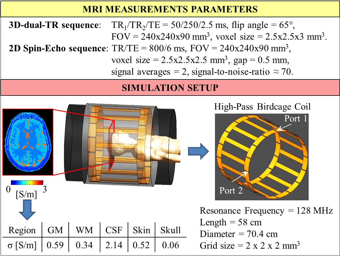
MRI measurements were performed on eight healthy volunteers (mean age 21.7, standard deviation 2.3) using a 3T MR-scanner (Achieva, Philips, Best, NL) and a 8-channel transmit/receive head coil. Conductivity reconstructions were performed according to[7]: σ(r)=Im((ΔB1+(r))/B1+(r))/μ0ω, with ω=Larmor frequency, μ0=free space permeability, and r=x,y,z-coordinates.The B1+ magnitude was measured using a 3D-dual-TR sequence8 (Figure 1).
For the B1+ phase, the transceive phase approximation was employed[9] by combining two phase maps acquired using 2D-single-echo Spin-Echo sequences with opposite readout gradient polarities (Figure 1). Gibbs-ringing correction and k-space Gaussian apodization were performed to minimize the impact of undesired high frequency spatial fluctuations[7].
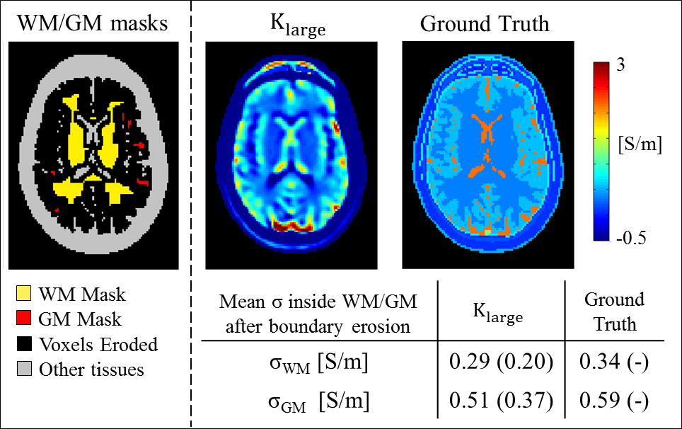
Second order spatial derivatives were computed using a large, noise-robust, in-plane derivative kernel (Klarge: 7x7 voxels)[7]. An in-plane kernel had to be used since well-known random phase offsets between slices prevented correct computations of spatial derivatives through slices.
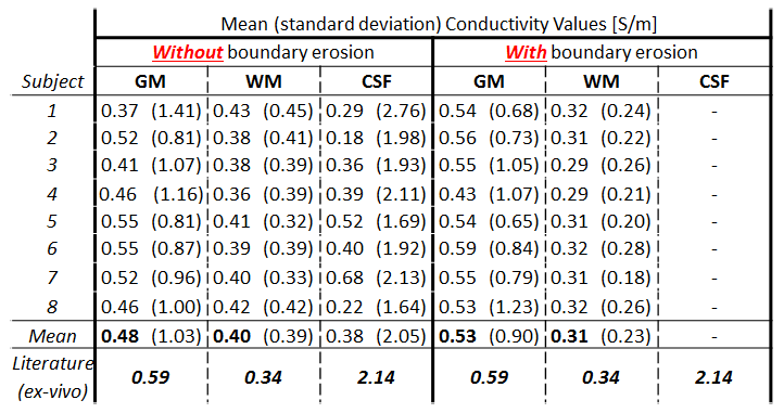
First, mean and standard deviation of σWM, σGM, and σCSF were computed for each subject. Tissue segmentation was performed in SPM12 using the Spin-Echo magnitude volumes. Only the voxels with a probability value (P) > 99% to belong to a certain tissue were considered, thus avoiding voxels with partial volumes.
Then, mean and standard deviation of σWM, σGM were computed for each subject after additional erosion (2 voxels erosion) of the WM and GM masks previously obtained from SPM12 was performed in order to avoid regions at tissue boundaries that are affected by typical MR-EPT boundary errors.
To benchmark the accuracy of these reconstructions, conductivity reconstructions were similarly performed using FDTD simulated complex B1+ data (Sim4Life, Duke head model, Figure 1), as simulated data allows knowledge of the ground truth conductivity. Gaussian noise was also included to mimic the SNR level obtained in the MR measurements. The mean σWM and σGM among 50 reconstructions with different noise realizations were computed over the whole head model, after the same in-plane erosion used for the in-vivo reconstructions was applied.
Results and Discussion
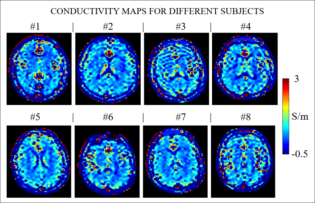
Figure 2 shows one slice of the reconstructed conductivity maps for the 8 subjects.Figure 3 shows that mean conductivity values are erroneous if boundary erosion is not performed. Instead, provided sufficient boundary erosion, mean σWM and σGM values are in good agreement with the reported literature values measured ex-vivo.
This indicates that:
1) boundary erosion is crucial for correct quantification of mean conductivity values;
2) the way boundaries are handled has severe impact on the reconstructed mean conductivity values.
This latter observation might be the reason why the few in-vivo data reported in literature are so different, as boundaries are differently handled among different studies.
Unfortunately, this erosion cannot be applied to the CSF due to its limited spatial extension. Smaller resolutions and small kernels should be adopted to correctly quantify σCSF, but this would lead to conductivity maps completely corrupted by noise. Hence, given the absence of a gold standard for in-vivo MR-EPT reconstructions, we believe that the agreement between σWM and σGM among eight subjects achieved in this work gives confidence on in-vivo σWM and σGM values for healthy subjects.
The results from simulations, performed to benchmark the accuracy of the reconstruction pipeline, are reported in Figure 4, where the reconstructed conductivity is shown for one slice, as well as the mean σWM and σGM values of the whole Duke head computed after the same erosion applied for the in-vivo conductivity reconstructions was performed. The mean σWM and σGM values among 50 reconstructions with different noise realizations agree with the reconstructed values in-vivo. However, these values show a small underestimation (~10%) with respect to the input ground truth. This is caused by the fact that the conductivity contribution arising from derivatives through slices are neglected, as these derivatives cannot be computed for the in-vivo case. This also explains the negligible underestimation in the reconstructed in-vivo σWM and σGM values with respect to literature ex-vivo values.
Conclusions
Boundary erosion is crucial to correctly quantify mean conductivity values. If boundaries are not handled correctly, erroneous mean conductivity values are obtained. This might explain the large variability among the brain conductivity values reported in literature.The in-vivo σWM and σGM values obtained in this study verify for the first time the literature values measured ex-vivo, while the accuracy of the reconstruction procedure was verified in simulation settings.
The presented σWM and σGM values can therefore be used as a verified reference for future studies where new reconstruction algorithms are tested in-vivo.
Acknowledgements
No acknowledgement found.References
1) Katscher U., van den Berg C.A.T., Electric properties tomography: Biochemical, physical and technical background, evaluation and clinical applications. NMRinBiomed 2017, DOI: 10.1002/nbm3729.
2) Hancu I., Liu J., Hua Y., Lee S.K., Electrical properties tomography: Available contrast and reconstruction capabilities. MRM 2018, DOI: 10.1002/mrm.27453.
3) Zhang X., Van de Moortele P.F., Schmitter S., He B.. Complex B1 mapping and electrical properties imaging of the human brain using a 16‐channel transceiver coil at 7T. MRM 2013, DOI: 10.1002/mrm.24358.
4) Voigt T., Katscher U., Doessel O.. Quantitative conductivity and permittivity imaging of the human brain using electric properties tomography. MRM 2011, DOI: 10.1002/mrm.22832.
5) Huhndorf M., Stehning C., Rohr A., et al., Systematic Brain Tumor Conductivity Study with Optimized EPT Sequence and Reconstruction Algorithm. ISMRM, Salt Lake City 2013. p. 3626.
6) Tha K.K., Katscher U., Yamaguchi S., et al. Noninvasive electrical conductivity measurement by MRI: a test of its validity and the electrical conductivity characteristics of glioma. European Radiology 2018: 348-355.
7) Mandija S., Sbrizzi A., Katscher U., Luijten P.R., van den Berg C.A.T.,Error analysis of Helmholtz‐based MR‐electrical properties tomography. MRM 2018, DOI: 10.1002/mrm.27004.
8) Yarnykh, V. L.. Actual flip‐angle imaging in the pulsed steady state: A method for rapid three‐dimensional mapping of the transmitted radiofrequency field. MRM 2007, DOI: 10.1002/mrm.21120.
9) van Lier A., Brunner D.O., Pruessmann K.P., Klomp D.W., Luijten P.R., Lagendijk J.J., van den Berg C.A.T.. B1+ Phase mapping at 7 T and its application for in vivo electrical conductivity mapping. MRM 2012, DOI: 10.1002/mrm.22995.
10) SPM12, WTCN, UCL, London, UK
Figures