Introduction

Electrical properties tomography (EPT) noninvasively retrieves conductivity and permittivity distributions in a patient’s body using a radio-frequency (RF) magnetic field ($$$H^+:=(H_x+iH_y)/2$$$) measured by B1 mapping¹. To improve the standard-MREPT (std-MREPT) (Katcher et al.)² assuming local homogeneity of electrical properties (EPs), various EPT methods were developed, accounting for spatial variations of EPs. The convection-reaction-MREPT³ (cr-MREPT) method solved partial differential equations (PDE) for the reciprocal of admittivity, $$$1/\gamma$$$. This can be obtained by eliminating $$$\bf{E}$$$ in Ampere’s law $$$\nabla\times\bf{H}=\gamma\bf{E}$$$ and using Faraday’s law $$$\nabla\times{\bf{E}}=-i\omega\mu\bf{H}$$$. As the Laplacian of $$$\bf{H}$$$ is required, cr-MREPT method is sensitive to noise. Iterative EPT^4,5 methods have been proposed using three-dimensional integral equations (IE) for the scattered field, without a Laplacian. We, however, devised complex-analysis-based Laplacian-free EPT methods^6,7. We first estimated $$$E_z$$$ by solving Faraday’s law as the first order PDE for $$$E_z$$$, given $$$H^+$$$ in the Region of Interest (ROI) with $$$\gamma$$$ on its boundary. We then calculated $$$\gamma$$$ by substituting the estimated $$$E_z$$$ into Ampere’s law. Note that these calculations relied on complex analysis formulae which hold in two-dimensional sub-ROIs sliced out of the original three-dimensional ROI. This required initial omission of $$$\partial_zH^+$$$ or $$$\partial_z\gamma$$$ for explicit calculation of $$$E_z$$$ on each slice. This must be followed by iterative calculations as post-processing in the final EP reconstruction for compensating those ignored terms. The proposed three-dimensional EPT method directly solves a newly derived IE, requiring no iterative calculations.

Method

In our previous method⁶, we estimated $$$E_z$$$ on each slice with the following two-dimensional IE under the assumption $$$\partial_zH^+=0$$$ :
$$\begin{align}E_z(w)=-\frac{1}{\pi}\int_{\Gamma}{\frac{2\partial H^+(\zeta)/\gamma(\zeta)}{\zeta-w}}d\zeta-\frac{\omega\mu}{\pi}\int\int_D{\frac{H^+(\zeta)}{\zeta-w}}d\xi d\eta,\notag\end{align}$$
where $$$\partial:=(\partial_x - i\partial_y)/2$$$, and $$$\gamma:=\sigma+i \omega\epsilon$$$. The term $$$\omega/2\pi$$$ is the Larmor frequency and $$$\sigma$$$ and $$$\epsilon$$$ are the conductivity and the permittivity, respectively. In order to estimate $$$\bf{E}$$$ inside ROI using our new method, without assumption $$$\partial_zH^+=0$$$, using Faraday’s law, Ampere’s law and vector calculus identities, we have derived
$$\begin{align}&{\bf{E}}({\bf{r}}')=-\frac{3}{2}\biggl(\int_{\partial\Omega}\left({\bf{n}}\times\frac{1}{\gamma}(\nabla\times{\bf{H}}({\bf{r}}))\right)\times\nabla\frac{1}{4\pi|{\bf{r}}-{\bf{r}}'|}dS+\lim_{\epsilon\rightarrow0} \int_{\Omega\backslash V_{\epsilon}}{\bigl({\bf{E}}({\bf{r}})\cdot\nabla+i\omega\mu{\bf{H}}({\bf{r}})\times\bigr)\nabla\frac{1}{4\pi|{\bf{r}}-{\bf{r}}'|}}dV\biggr),\notag\end{align}$$
where $$$V_{\epsilon}$$$ is the infinitesimal cubic volume domain surrounding $$$\bf{r}$$$ with sides of length $$$\epsilon$$$. Note that $$$V_{\epsilon}$$$ must be cubic to establish this equation. Incorporating the three assumptions, $$$H_z=0$$$, $$$|H^-|\ll|H^+|$$$ and $$$\gamma$$$ being known on the boundary of ROI, the following approximation about the above equation holds:
$$\begin{align}&{\bf{E}}({\bf{r}}') +\frac{3}{2}\Biggl(\lim_{\epsilon\rightarrow0}\int_{\Omega\backslash V_{\epsilon}}{{\bf{E}}\cdot\nabla \nabla\frac{1}{4\pi|{\bf{r}}-{\bf{r}}'|}}\,dV\Biggr)\notag\\ &=-\frac{3}{2}\Biggl(\int_{\partial\Omega}\biggl({\bf{n}}\times\frac{1}{\gamma} \begin{bmatrix} -i\partial_zH^+\\ \partial_zH^+\\ -4i\partial H^+ \end{bmatrix} \biggr)\times\nabla\frac{1}{4\pi|{\bf{r}}-{\bf{r}}'|}\,dS +\lim_{\epsilon\rightarrow0}\int_{\Omega\backslash V_{\epsilon}}{i\omega\mu \begin{bmatrix} H^+\\ -iH^+\\ 0 \end{bmatrix} \times\nabla\frac{1}{4\pi|{\bf{r}}-{\bf{r}}'|}}\,dV\Biggr)=:{\bf{C}}({\bf{r}}').\notag \end{align}$$
In this equation, $$$\bf{E}$$$ on the left side is unknown whereas the integrals on the right side can be computed from the measured $$$H^+$$$ and $$$\gamma$$$ on the boundary. The above equation can be discretized to the following linear equation:
$$\begin{align}A{\bf{e}}={\bf{c}},\notag\end{align}$$
where $$$\bf{e}$$$ and $$$\bf{c}$$$ are the vectors corresponding with $$$\bf{E}$$$ and $$$\bf{C}$$$ at each sampled point, and $$$A$$$ is the matrix determined by this discretization. We can estimate $$$\bf{E}$$$ by solving this linear equation with Tikhonov regularization, and then calculate $$$\gamma$$$ from $$$E_z$$$ using Ampere’s law. $$$E_x$$$ and $$$E_y$$$ are not used here because their magnitudes are smaller than $$$E_z$$$ resulting in deteriorated accuracy when using MRI.

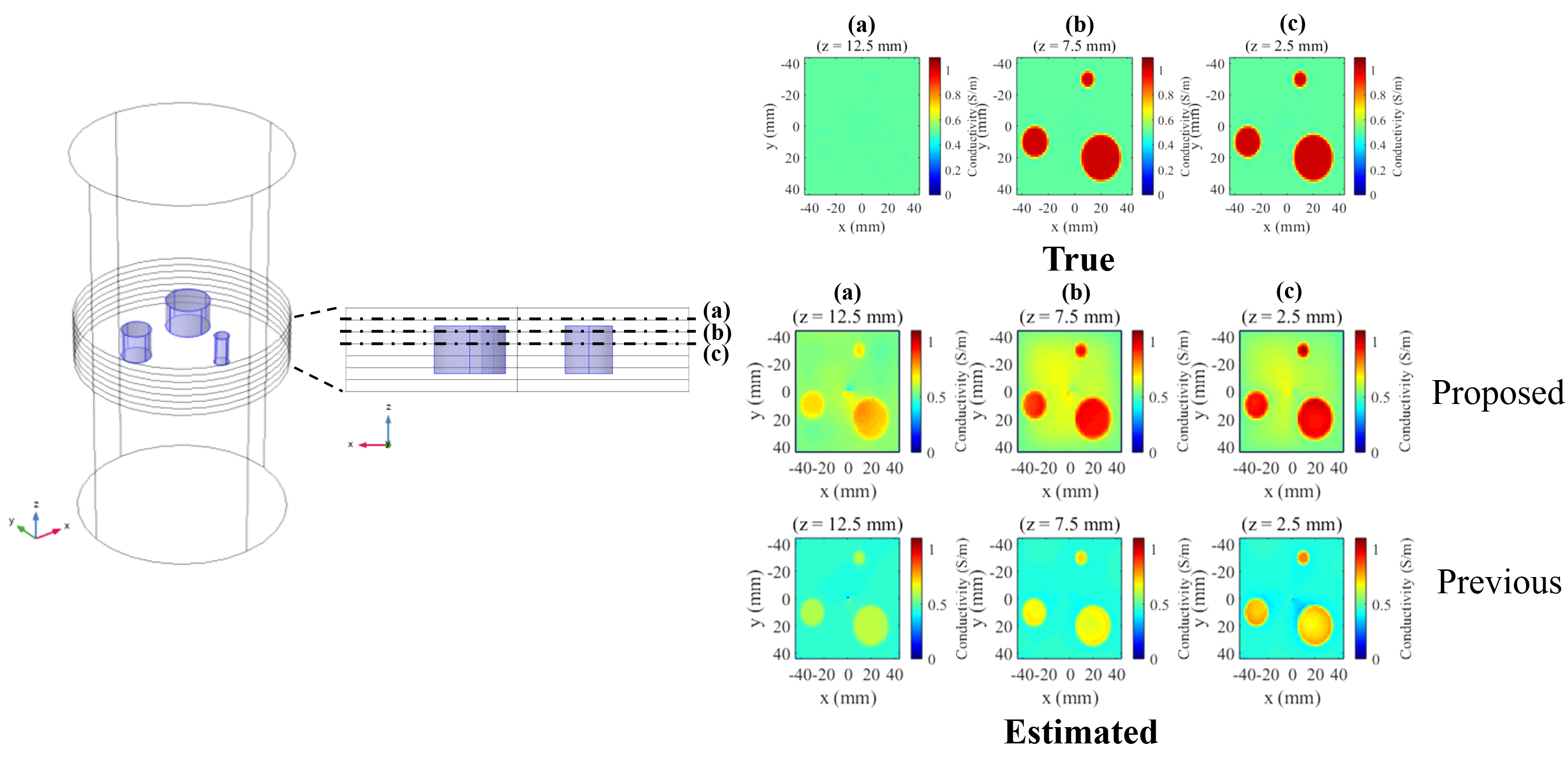
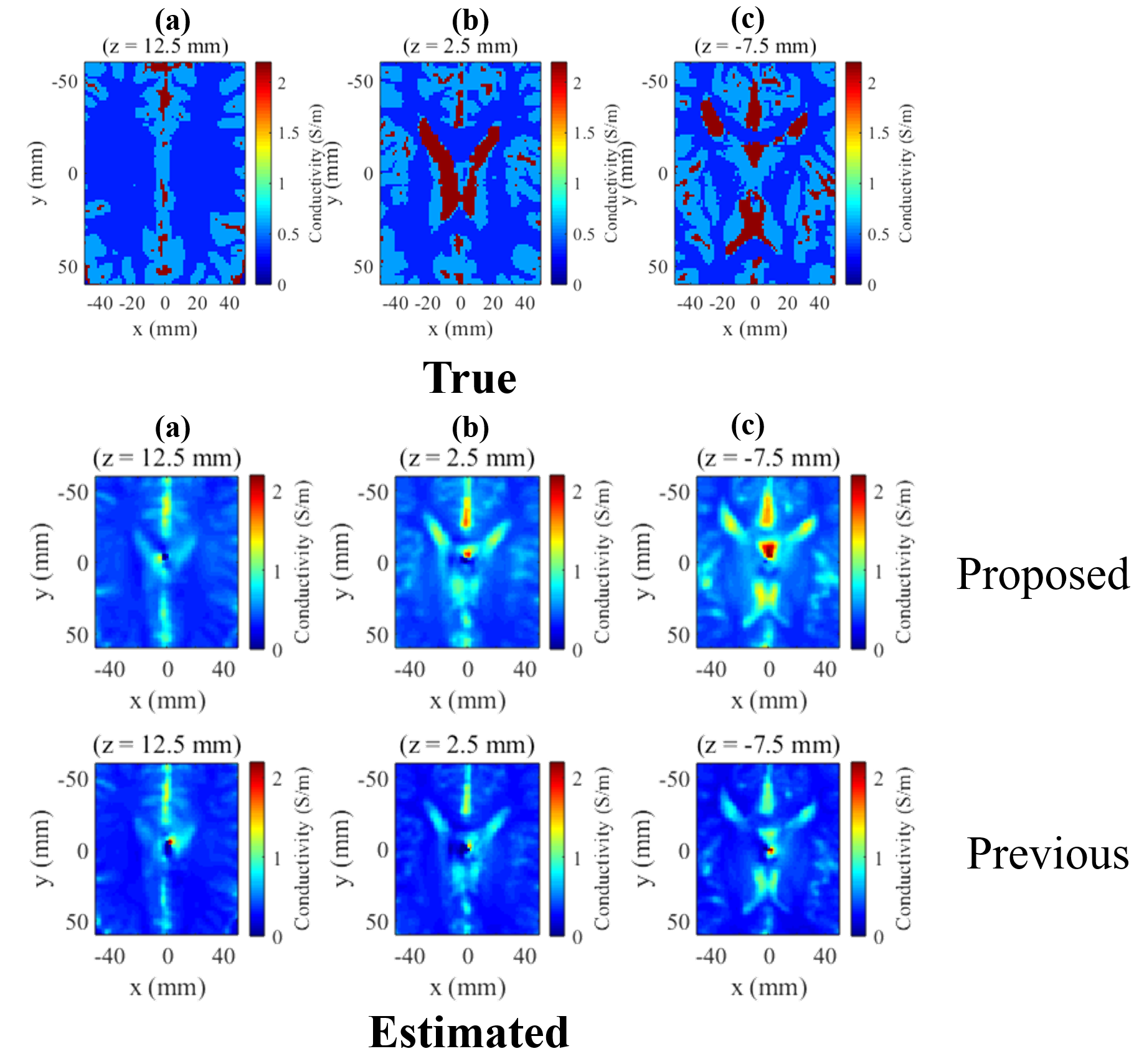
We verified our method using numerical simulations and a phantom experiment using 3T MR scanner (Siemens, Magnetom Prisma). In the simulations $$$H^+$$$ data was computed using FEM software (COMSOL Multiphysics, COMSOL Inc.). The following two situations were modeled: Model 1 was a simple model including three cylindrical regions of higher conductivity ($$$\sigma$$$ = 1.0 S/m) than the background material ($$$\sigma$$$ = 0.5 S/m). Model 2 was a head model (Aubert-Broche et al)⁸. We compared the proposed method with our previous method⁶ ignoring $$$\partial_zH^+$$$ without iteration.

Results&Discussion

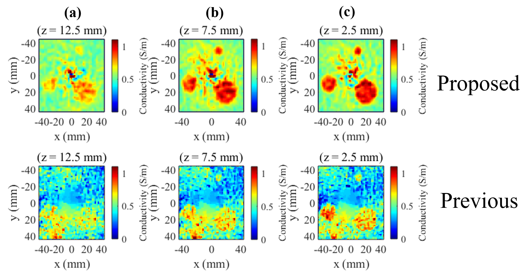
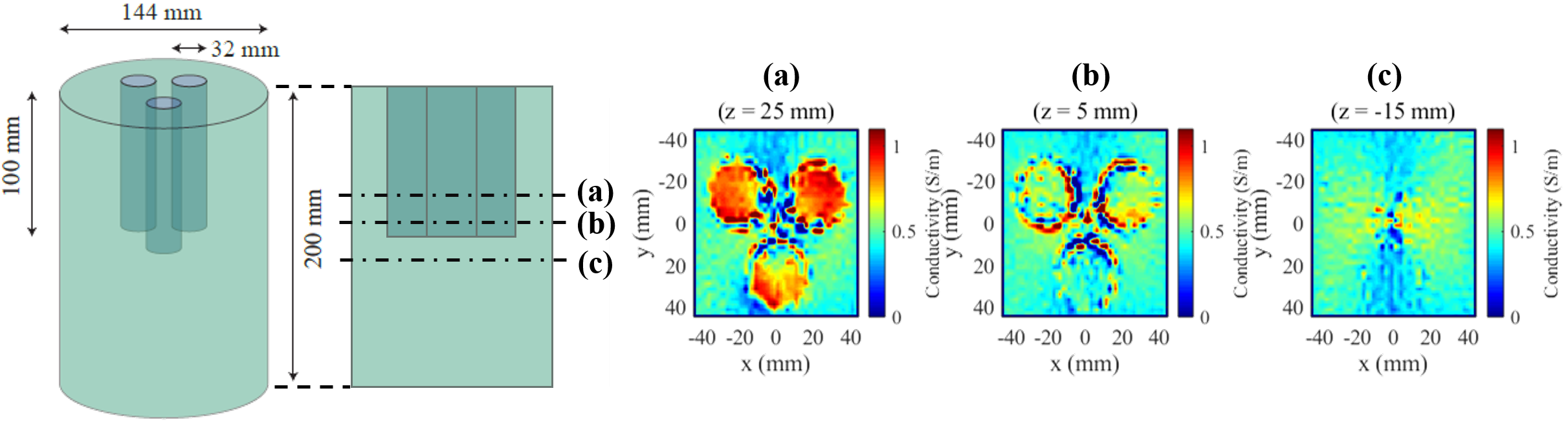
Figure 1 shows the reconstruction results of model 1. The proposed method can reconstruct conductivity values with greater accuracy, by removing presumed vertical uniformity of EPs and $$$H^+$$$. With 5% Gaussian noise added, the proposed method remains stable (Figure 2). A possible factor for this is the larger integral domain in the proposed method (three-dimensional) than that in the previous method (two-dimensional). The proposed method also outperformed the previous method with model 2 (Figure 3). In the phantom experiment results (Figure 4), we see the three high-conductivity regions clearly distinguished from the background. However, challenges exist in the accurate estimation of absolute conductivity values, especially in regions where $$$E_z$$$ discontinuously varied along the $$$z$$$-axis. To solve this, use of $$$E_x$$$ and $$$E_y$$$ for reconstruction will be addressed in future studies.

Conclusion

In this paper, we presented a novel, noniterative three-dimensional EPT method based on the computation of the electric field via the newly derived IE. The results indicate that EP reconstruction using the proposed method had greater accuracy and robustness against noise than the previous method.

Acknowledgements

This research was supported in part by JPSP KAKENHI Grant Number 19H04438 and Canon Medical Systems Corporation.